Lecture 12(1)
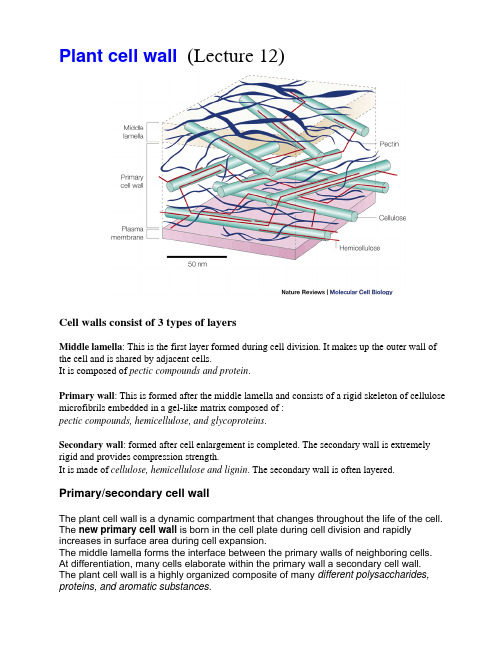
Plantcellwall(Lecture12)
Cell walls also contain functional proteins. Enzymatic activities in cell walls include: •Oxidative enzymes - peroxidases•Hydrolytic enzymes - pectinases, cellulases•"Expansins" - enzymes that catalyze cell wall "creep" activity General functions of cell wall enzymes include:
galacturonic acid
Pectic acid with salt bridges
4. Pectin - polymer of around 200 galacturonic acid molecules - many of the carboxyl groups are methylated (COOCH3) - less hydrated then pectic acid but soluble in hot water - another major component of middle lamella but also found in primary walls
lecture12
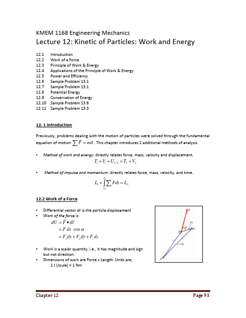
KMEM 1168 Engineering MechanicsLecture 12: Kinetic of Particles: Work and Energy12.1 Introduction 12.2 Work of a Force12.3 Principle of Work & Energy12.4 Applications of the Principle of Work & Energy 12.5 Power and Efficiency 12.6 Sample Problem 13.1 12.7 Sample Problem 13.1 12.8 Potential Energy12.9 Conservation of Energy 12.10 Sample Problem 13.6 12.11 Sample Problem 13.312. 1 IntroductionPreviously, problems dealing with the motion of particles were solved through the fundamentalequation of motion a m F rr =∑. This chapter introduces 2 additional methods of analysis.•Method of work and energy : directly relates force, mass, velocity and displacement. 222111V T U V T +=++−•Method of impulse and momentum : directly relates force, mass, velocity, and time.2121L Fdt L t t =+∫∑12.2 Work of a Force• Differential vector dr is the particle displacement •Work of the force isdzF dy F dx F ds F rd F dU z y x ++==•=αcos r r• Work is a scalar quantity, i.e., it has magnitude and sign but not direction.• Dimensions of work are Force x Length. Units are,1 J (Joule) = 1 Nm• Work of a force during a finite displacement,• Work is represented by the area under the curve of F t plotted against s .• Work of a constant force in rectilinear motion,•Forces which do not do work (ds = 0 or cos a = 0):a) reaction at frictionless pin supporting rotating bodyb) reaction at frictionless surface when body in contact moves along surface c) weight of a body when its center of gravity moves horizontally12.3 Principle of Work & Energy•Consider a particle of mass m acted upon by a force•Integrating from A 1to A 2,•The work of the force is equal to the change in kinetic energy of the particle.• Units of work and kinetic energy are the same:12.4 Applications of the Principle of Work & Energy•The bob is held at point 1 and if we wish to find the velocity of pendulum bob at point 2, we have to consider the method of work and energy. Force P acts normal to path and does no work.•In this method, unlike the method of Newton 2nd Law, we can find velocity without having to determine expression for acceleration and integrating.•All quantities are scalars and can be added directly. Forces which do no work (eg. In this case is the tension in the cord P)are eliminated from the problem. Principle of work and energy cannot be applied to directly determine the acceleration of the pendulum bob.•The tension in the cord is required to supplement the method of work and energy with an application of Newton’s second law.•As the bob passes through A 2,12.5 Power and Efficiency•Power = rate at which work is done.vF dt r d F dt dU r r r r •=•==•Dimensions of power are work/time or force x velocity. Units for power are• Efficiency is the ratio of the power output to the power input,12.6 Sample Problem 13.1An automobile weighing 4000 N is driven down a 5oincline at a speed of 88 m /s when the brakes are applied causing a constant total breaking force of 1500 N.Determine the distance traveled by the automobile as it comes to a stop.• Evaluate the change in kinetic energy.()()m N 15488008810/4000sm 88221212111⋅====mv T v0022==T v•Determine the distance required for the work to equal the kinetic energy change.()()()()x x x U 11515sin 4000150021−=°+−=→()0115115488002211=−=+→x T U Tm 6.1345=x12.7 Sample Problem 13.2Two blocks are joined by an inextensible cable as shown. If the system is released from rest, determine the velocity of block A after it has moved 2 m.Assume that the coefficient of friction between block A and the plane is μk= 0.25 and that the pulley isweightless and frictionless.• Apply the principle of work and energy separately to blocks A and B .Block A:()()()()()()()()()221221221120024902220:N490196225.0N 196281.9200v F vm F F T U T W N F W C A A C A k A k A A =−=−+=+======→µµBlock B:()()()()()()()()2212212211300229402220:N 294081.9300v F vm W F T U T W c B B c B =+−=+−=+==→•When the two relations are combined, the work of the cable forces cancel. Solve for the velocity.()()()()22120024902v F C =−()()()()221300229402v F c =+−()()()()()()2212215004900300200249022940vv=+=− s m 43.4=v12.8 Potential EnergyThere are 2 kinds of potential energyi) Gravitational Potential Energy, V g ii) Elastic Potential Energy, V eGravitational Potential Energy (V g )• Work of the force of gravity W ,2121y W y W U −=→• Work is independent of path followed, it depends only on the initial and final values of W(dy).()()2121g g V V U −=→•Choice of datum from which the elevation y is measured is arbitrary. But always choose the lower position as the datum to avoid negative potential energy. Units of work and potential energy are the same:J m N )(=⋅==dy W V gElastic Potential Energy, V e• Work of the force exerted by a spring dependsonly on the initial and final deflections of the spring,2221212121kx kx U −=→• The potential energy of the body with respect tothe elastic force,()()2121221e e e V V U kxV −==→•Note that the preceding expression for V e is valid only if the deflection of the spring is measured from its undeformed position.=→21U 221kx12.9 Conservation of Energy•Conservation of energy equation,constant2211=+=+=+V T E V T V T• When a particle moves under the action of conservative forces, the total mechanical energy (E) is constant.•Friction forces are not conservative. Total mechanical energy of a system involving friction decreases. Mechanical energy is dissipated by friction into thermal energy or heat.ll W V T W V T =+==11110()ll l W V T V W g g Wmv T =+====22222212022112.10 Sample Problem 13.6A 20-N collar slides without friction along a vertical rod as shown. The spring attached to the collar has an undeflected length of 4 cm and a constant of 3 N/cm. If the collar is released from rest at position 1, determine its velocity after it has moved 6 cm to position 2.• Apply the principle of conservation of energy betweenpositions 1 and 2.Position 1:()()0024cmN 24483112212121=+=+=⋅=−==T V V V kx V g e ePosition 2:()()()()222221222212221102021cm N 6612054cmN 120620cmN 544013v mv T V V V Wy V kx V g e g e ==⋅−=−=+=⋅−=−==⋅=−==•Conservation of Energy:cmN 66cm N 240222211⋅−=⋅++=+v V T V T↓=s m 5.92v12.11 Sample Problem 13.3A spring is used to stop a 60 kg package which is sliding on a horizontal surface. The spring has a constant k = 20 kN/m and is held by cables so that it is initially compressed 120 mm. The package has a velocity of 2.5 m/s in the position shown and the maximum deflection of the spring is 40 mm. Determine(a) the coefficient of kinetic friction between the package and surface(b) the velocity of the package as it passes again through the position shown.(a) Use principle of work and energy equation,NF g N µ==60222111V T U V T +=++→021)(212122212+∆=−∆+x k s N x k mu µ()()222)04.012.0)(20000(2)04.06.0)(60()12.0)(20000(215.26021+=+−+g µ 20.0=µ(b) Apply the principle of work and energy for the rebound of the package.333222V T U V T +=++→ 2323222121)(210x k mv s N x k ∆+=−∆+µ2232)12.0)(20000(21)60(21)64.0)(60)(2.0()16.0)(20000(21+=−v g s m v /11.13=NB: Part B demonstrates that the final velocity at 3 is less than the initial velocity at 1. This is due to the loss of energy due to friction. The total mechanical energy is not conserved.。
cs231n_2017_lecture12

Lecture 12: Visualizing and UnderstandingAdministrativeMilestones due tonight on Canvas, 11:59pmMidterm grades released on Gradescope this weekA3 due next Friday, 5/26HyperQuest deadline extended to Sunday 5/21, 11:59pm Poster session is June 6Last Time: Lots of Computer Vision TasksClassification + LocalizationSemantic SegmentationObject DetectionInstance SegmentationCATGRASS , CAT , TREE , SKYDOG , DOG , CATDOG , DOG , CATSingle ObjectMultiple ObjectNo objects, just pixelsThis image is CC0 public domainThis image is CC0 public domainWhat’s going on inside ConvNets?This image is CC0 public domainClass Scores:1000 numbers Input Image:3 x 224 x 224What are the intermediate features looking for?Krizhevsky et al, “ImageNet Classification with Deep Convolutional Neural Networks”, NIPS 2012.Figure reproduced with permission.First Layer: Visualize FiltersAlexNet:64 x 3 x 11 x 11ResNet-18:64 x 3 x 7 x 7ResNet-101:64 x 3 x 7 x 7DenseNet-121:64 x 3 x 7 x 7Krizhevsky, “One weird trick for parallelizing convolutional neural networks”, arXiv 2014 He et al, “Deep Residual Learning for Image Recognition”, CVPR 2016Huang et al, “Densely Connected Convolutional Networks”, CVPR 2017Visualize the filters/kernels (raw weights)We can visualize filters at higher layers, but not that interesting (these are taken from ConvNetJS CIFAR-10 demo)layer 1 weightslayer 2 weightslayer 3 weights16 x 3 x 7 x 720 x 16 x 7 x 720 x 20 x 7 x 7FC7 layerLast Layer4096-dimensional feature vector for an image (layer immediately before the classifier)Run the network on many images, collect the feature vectorsLast Layer: Nearest Neighbors4096-dim vectorTest image L2 Nearest neighbors in feature spaceRecall: Nearest neighborsin pixel spaceKrizhevsky et al, “ImageNet Classification with Deep Convolutional Neural Networks”, NIPS 2012.Figures reproduced with permission.Visualize the “space” of FC7 feature vectors by reducing dimensionality of vectors from 4096 to 2 dimensionsSimple algorithm: Principle Component Analysis (PCA) More complex: t-SNEVan der Maaten and Hinton, “Visualizing Data using t-SNE”, JMLR 2008Figure copyright Laurens van der Maaten and Geoff Hinton, 2008. Reproduced with permission.Van der Maaten and Hinton, “Visualizing Data using t-SNE”, JMLR 2008Krizhevsky et al, “ImageNet Classification with Deep Convolutional Neural Networks”, NIPS 2012. Figure reproduced with permission.See high-resolution versions at/people/karpathy/cnnembed/Visualizing ActivationsYosinski et al, “Understanding Neural Networks Through Deep Visualization”, ICML DL Workshop 2014.Figure copyright Jason Yosinski, 2014. Reproduced with permission.conv5 feature map is128x13x13; visualizeas 128 13x13grayscale imagesMaximally Activating PatchesPick a layer and a channel; e.g. conv5 is128 x 13 x 13, pick channel 17/128Run many images through the network,record values of chosen channelVisualize image patches that correspondto maximal activationsSpringenberg et al, “Striving for Simplicity: The All Convolutional Net”, ICLR Workshop 2015Figure copyright Jost Tobias Springenberg, Alexey Dosovitskiy, Thomas Brox, Martin Riedmiller, 2015;reproduced with permission.Occlusion Experiments Mask part of the image beforefeeding to CNN, draw heatmap ofprobability at each mask locationZeiler and Fergus, “Visualizing and Understanding Convolutional Networks”, ECCV 2014Boat image is CC0 public domain Elephant image is CC0 public domain Go-Karts image is CC0 public domainHow to tell which pixels matter for classification?Dog Simonyan, Vedaldi, and Zisserman, “Deep Inside Convolutional Networks: Visualising Image Classification Modelsand Saliency Maps”, ICLR Workshop 2014.Figures copyright Karen Simonyan, Andrea Vedaldi, and Andrew Zisserman, 2014; reproduced with permission.How to tell which pixels matter for classification?Dog Compute gradient of (unnormalized) classscore with respect to image pixels, takeabsolute value and max over RGB channelsSimonyan, Vedaldi, and Zisserman, “Deep Inside Convolutional Networks: Visualising Image Classification Modelsand Saliency Maps”, ICLR Workshop 2014.Figures copyright Karen Simonyan, Andrea Vedaldi, and Andrew Zisserman, 2014; reproduced with permission.Simonyan, Vedaldi, and Zisserman, “Deep Inside Convolutional Networks: Visualising Image Classification Models and Saliency Maps”, ICLR Workshop 2014.Figures copyright Karen Simonyan, Andrea Vedaldi, and Andrew Zisserman, 2014; reproduced with permission.Saliency Maps: Segmentation without supervision Simonyan, Vedaldi, and Zisserman, “Deep Inside Convolutional Networks: Visualising Image Classification Modelsand Saliency Maps”, ICLR Workshop 2014.Figures copyright Karen Simonyan, Andrea Vedaldi, and Andrew Zisserman, 2014; reproduced with permission.Rother et al, “Grabcut: Interactive foreground extraction using iterated graph cuts”, ACM TOG 2004Use GrabCut onsaliency mapPick a single intermediate neuron, e.g. onevalue in 128 x 13 x 13 conv5 feature mapCompute gradient of neuron value with respectto image pixelsZeiler and Fergus, “Visualizing and Understanding Convolutional Networks”, ECCV 2014Springenberg et al, “Striving for Simplicity: The All Convolutional Net”, ICLR Workshop 2015Pick a single intermediate neuron, e.g. onevalue in 128 x 13 x 13 conv5 feature mapCompute gradient of neuron value with respectto image pixelsImages come out nicer if you onlybackprop positive gradients througheach ReLU (guided backprop)ReLUZeiler and Fergus, “Visualizing and Understanding Convolutional Networks”, ECCV 2014 Springenberg et al, “Striving for Simplicity: The All Convolutional Net”, ICLR Workshop 2015Figure copyright Jost Tobias Springenberg, Alexey Dosovitskiy, Thomas Brox, Martin Riedmiller, 2015; reproduced with permission.Zeiler and Fergus, “Visualizing and Understanding Convolutional Networks”, ECCV 2014Springenberg et al, “Striving for Simplicity: The All Convolutional Net”, ICLR Workshop 2015Figure copyright Jost Tobias Springenberg, Alexey Dosovitskiy, Thomas Brox, Martin Riedmiller, 2015; reproduced with permission.(Guided) backprop: Find the part of an image that a neuron responds to Gradient ascent: Generate a synthetic image that maximally activates a neuronI* = arg maxIf(I) + R(I)Neuron value Natural image regularizer1.Initialize image to zerosscore for class c (before Softmax) zero imageRepeat:2. Forward image to compute current scores3. Backprop to get gradient of neuron value with respect to image pixels4. Make a small update to the imageSimple regularizer: Penalize L2norm of generated imageSimonyan, Vedaldi, and Zisserman, “Deep Inside Convolutional Networks: Visualising Image Classification Models and Saliency Maps”, ICLR Workshop 2014.Figures copyright Karen Simonyan, Andrea Vedaldi, and Andrew Zisserman, 2014; reproduced with permission.Simple regularizer: Penalize L2norm of generated imageSimonyan, Vedaldi, and Zisserman, “Deep Inside Convolutional Networks: Visualising Image Classification Models and Saliency Maps”, ICLR Workshop 2014.Figures copyright Karen Simonyan, Andrea Vedaldi, and Andrew Zisserman, 2014; reproduced with permission.Simple regularizer: Penalize L2norm of generated imageYosinski et al, “Understanding Neural Networks Through Deep Visualization”, ICML DL Workshop 2014. Figure copyright Jason Yosinski, Jeff Clune, Anh Nguyen, Thomas Fuchs, and Hod Lipson, 2014. Reproduced with permission.Better regularizer: Penalize L2 norm of image; also during optimization periodically(1)Gaussian blur image(2)Clip pixels with small values to 0(3)Clip pixels with small gradients to 0 Yosinski et al, “Understanding Neural Networks Through Deep Visualization”, ICML DL Workshop 2014.Better regularizer: Penalize L2 norm ofimage; also during optimizationperiodically(1)Gaussian blur image(2)Clip pixels with small values to 0(3)Clip pixels with small gradients to 0Yosinski et al, “Understanding Neural Networks Through Deep Visualization”, ICML DL Workshop 2014.Figure copyright Jason Yosinski, Jeff Clune, Anh Nguyen, Thomas Fuchs, and Hod Lipson, 2014. Reproduced with permission.Better regularizer: Penalize L2 norm ofimage; also during optimizationperiodically(1)Gaussian blur image(2)Clip pixels with small values to 0(3)Clip pixels with small gradients to 0Yosinski et al, “Understanding Neural Networks Through Deep Visualization”, ICML DL Workshop 2014.Figure copyright Jason Yosinski, Jeff Clune, Anh Nguyen, Thomas Fuchs, and Hod Lipson, 2014. Reproduced with permission.Use the same approach to visualize intermediate featuresYosinski et al, “Understanding Neural Networks Through Deep Visualization”, ICML DL Workshop 2014.Figure copyright Jason Yosinski, Jeff Clune, Anh Nguyen, Thomas Fuchs, and Hod Lipson, 2014. Reproduced with permission.Use the same approach to visualize intermediate featuresYosinski et al, “Understanding Neural Networks Through Deep Visualization”, ICML DL Workshop 2014.Figure copyright Jason Yosinski, Jeff Clune, Anh Nguyen, Thomas Fuchs, and Hod Lipson, 2014. Reproduced with permission.Adding “multi-faceted” visualization gives even nicer results:(Plus more careful regularization, center-bias)Nguyen et al, “Multifaceted Feature Visualization: Uncovering the Different Types of Features Learned By Each Neuron in Deep Neural Networks”, ICML Visualization for Deep Learning Workshop 2016. Figures copyright Anh Nguyen, Jason Yosinski, and Jeff Clune, 2016; reproduced with permission.Figures copyright Anh Nguyen, Jason Yosinski, and Jeff Clune, 2016; reproduced with permission.Optimize in FC6 latent space instead of pixel space:Nguyen et al, “Synthesizing the preferred inputs for neurons in neural networks via deep generator networks,” NIPS 2016Figure copyright Nguyen et al, 2016; reproduced with permission.(1)Start from an arbitrary image(2)Pick an arbitrary class(3)Modify the image to maximize the class(4)Repeat until network is fooledBoat image is CC0 public domain Elephant image is CC0 public domainWhat is going on? Ian Goodfellow will explain Boat image is CC0 public domainElephant image is CC0 public domainRather than synthesizing an image to maximize a specific neuron, insteadtry to amplify the neuron activations at some layer in the networkChoose an image and a layer in a CNN; repeat:1.Forward: compute activations at chosen layer2.Set gradient of chosen layer equal to its activation3.Backward: Compute gradient on image4.Update imageMordvintsev, Olah, and Tyka, “Inceptionism: Going Deeper into NeuralNetworks”, Google Research Blog. Images are licensed under CC-BY4.0Rather than synthesizing an image to maximize a specific neuron, instead try to amplify the neuron activations at some layer in the networkEquivalent to:I* = arg max I ∑i f i (I)2Mordvintsev, Olah, and Tyka, “Inceptionism: Going Deeper into Neural Networks”, Google Research Blog . Images are licensed under CC-BY 4.0Choose an image and a layer in a CNN; repeat:1.Forward: compute activations at chosen layer 2.Set gradient of chosen layer equal to its activation 3.Backward: Compute gradient on image 4.Update imageCode is very simple but it uses a couple tricks: (Code is licensed under Apache 2.0)Code is very simple but it uses a couple tricks: (Code is licensed under Apache 2.0)Jitter imageCode is very simple but it uses a couple tricks: (Code is licensed under Apache 2.0)Jitter imageL1 Normalize gradientsCode is very simple butit uses a couple tricks:(Code is licensed under Apache 2.0)Jitter imageL1 Normalize gradientsClip pixel valuesAlso uses multiscale processing for a fractal effect (not shown)Sky image is licensed under CC-BY SA 3.0Image is licensed under CC-BY 4.0Image is licensed under CC-BY 4.0Image is licensed under CC-BY 3.0Image is licensed under CC-BY 3.0Image is licensed under CC-BY 4.0Given a CNN feature vector for an image, find a new image that: -Matches the given feature vector-“looks natural” (image prior regularization)Mahendran and Vedaldi, “Understanding Deep Image Representations by Inverting Them”, CVPR 2015Given feature vectorFeatures of new imageTotal Variation regularizer (encourages spatial smoothness)Reconstructing from different layers of VGG-16Mahendran and Vedaldi, “Understanding Deep Image Representations by Inverting Them”, CVPR 2015Figure from Johnson, Alahi, and Fei-Fei, “Perceptual Losses for Real-Time Style Transfer and Super-Resolution”, ECCV 2016. Copyright Springer, 2016.Reproduced for educational purposes.。
lecture12(I) 导体上电磁波的传播

0
4ki
ki2 kr2
4ki
α
2 f
0
ki
kr
1
PL
1
2
α
2 f
0
P I2R
导体表面上的反射 1.电磁波由真空垂直入
射于导体表面
E E' E"
H H' H"
2.幅值关系
'" 0
" 导体
k" H"
真空
'
k
k'
H H'
真空中:H
0 n E H, E
0
同相位
H E
0 0
H 0 0 E H ' 0 0 E'
krz
1 2
2
1
2 2
11 2
12
kiz
1 2
1
2 2
2
1
d.良导体中的 k kr iki
良导体
1 ωLeabharlann k 2 2( i ) i
k i
kr ki
2
利用2c可得相同结果
12
kr z
1 2
1
2 22
1
1 ω
kr
2
12
kiz
1 2
i
e4 nE
2
H 与 E 相位相差 4
d.
良导体
一般均匀介质
电场与磁 场关系
电场与磁 场相位差
幅值比
HE
H
i
e4 nE
H 1 kE
4
H
i
e4
0
E
H E
H H EE
Lecture12-Language Acquisition

• Definition of “second language” (L2):
– Any language other than the first language learned (in a broader sense). – A language learned after the first language in a context where the language is used widely in the speech community (in a narrower sense). • e.g., For many people in Taiwan, their L1 is Taiwanese and L2 is Mandarin.
1) imitation (word-for-word repetition)
2) practice (repetitive manipulation of form)
3) feedback on success (positive reinforcement) 4) habit formation.
Lecture 12 cohesion andcoherence 英语词汇学 教学课件

Conjunctions
Conjuncts have a fundamental role in the cohesion of a text and may have various functions
Listing (indicating that what follows is a list of propositions) To start with, First, Second, Third
Chapter 12 Cohesion & Coherence
Revision Causes for Meaning Change in Words
1. Historical 2. Social 3. Psychological 4. linguistic
Pencil”, for instance, is from a Latin word meaning “a little tail” or “a fine brush”, like our Chinese “pen”. Later, when it was made of wood and graphite, it was still called a “pencil”. “Engine” originates in Latin word “ingenium, natural ability”. But when stream power was developed in the first quarter of the 19th century, the term “engine” comes to mean “a railroad locomotive”, and in contemporary English it means “any machine that uses energy to develop mechanical power, esp., a machine for starting motion in some other machine”
大数据分析与计算 第12课 GraphParallel图并行计算框架
Big Data Computing Technology
Lecture 12 图并行计算框架
图计算问题 BSP图计算模型 图计算架构
1
大数据计算技术
Big Data Computing Technology
图计算问题
2
大数据计算技术
Big Data Computing Technology路由器全时钟组件一组件二
组件三
图 13-9 BSP 逻辑结构组成
10
大数据计算技术
Big Data Computing Technology
BSP超步(Superstep)
BSP的核心思想是: 将任务分步完成,通过定义SuperStep (超步) 来完成任务的分步计算。也就是将一个大任务分解为一定数量的超步, 而在每一个超步内各计算节点(即组件,Virtual Processor代表) 独立 地完成本地的计算任务,将计算结果进行本地存储和远程传递以后, 在全局时钟的控制下进入下一个超步。
网络图计算
大型图(像社交网络和网络图等)常常作为系统计算的 一部分, 图计算问题包括最短路径、集群、网页排名、最小 切割、连通分支等。Google报道有20%数据是采用图计算 模型处理。
3
大数据计算技术
Big Data Computing Technology
图计算基本概念
图(graph):由非空顶点(vertex)集合V和边(edge) 集合E组成的二元组(V, E)称为图,记为G=(V,E)。
某些进程在特定的超步中 可以不必进行障碍同步(比 如在Superstep 0, Superstep 1之间,BSP Peer1与BSP Peer 2在遇到
Barrier Synchronizationer 1
Lecture-12[1]
1
Agenda • m-Logistics Service Demo • Web Services Development • Web Service Deployment • Web Service Trouble-shooting • Introduction to Milestone 4 • Course Logistics
13
How to create effective UI
User Interface Design, Anna Karpasov 14
Sample early UI wireframe
15
Courier
Homepage Notes: • Home base for all couriers, with mix of practical functionality (check-in, my money, jobs, barcode) and “fun” (leaders, ratings) • Notifications at bottom to alert of any important new activity
7
WS on the Backend Server
• Java – Axis2/Java – Example: /library/1719 • PHP – WSO2 PHP Framework – Example: /project/wsf/php/2.1.0/docs/ manual.html
24
Development Cycle
20
Agenda • m-Logistics Service Demo • Web Services Development • Web Service Deployment • Web Service Trouble-shooting • Introduction to Milestone 4 • Course Logistics
Lecture1 12关系分句-1
1 Relative clauses are also called attributive[ə'tribjutiv]定语的;归属 的/adjective clauses. They come after nouns and modify them. 2 They tell the listener or reader more about the person or thing that the noun refer to. 3 They can be divided into restrictive relative clauses and nonrestrictive relative clauses.
2. When the noun head takes a cataphoric [,kætə'fɔ:rik]前照 应definite article This is the car I bought last year.
3. When the noun head takes such indefinite determiners as some, any, no, all, every No visitors who come to Beijing would fail to see the Great Wall.
3. Ellipsis [i'lipsis]省略;省略符号;脱漏of relative words a) When a relative pronoun is used as object in the clause Tom is not the boy I gave the tickets to. b) When relative that is used as subject complement in an SVC construction, normally omitted He’s changed. He’s not the man he was. c) When the relative clause appears as part of It is/That is/There is construction, its subject can be omitted, only applies to informal style It isn’t everybody can learn a foreign language so easily. That was his brother just went by. There was someone asked for you, Bill.
中级微观成本最小化
如果厂商所选择的固定要素使用量恰好使长期 成本最小化,那么长期内使成本最小化的可变 要素使用量就是厂商短期内所选择的使用量。
x1(w1 , w2 , y) x1s[w1, w2 , x2 ( y), y]
22
示例:
厂商的生产函数为y=ALαKβ。生产要素L 和K的价格分别为wL,wK。
4
成本最小化
构造拉格朗日函数求解:
wx ( y f ( x))
一阶条件:wi
f ( xi ) , i xi
1,, n
任取其中的两种投入,变化后可得:
f ( x) / xi wi f ( x) / x j w j
5
边际替代率等于要素价格比率
成本最小化
等成本线斜率等于等产量线斜率,即
y f (x1*, x2*)
s.t. f (x1, x 2) y
短期要素需求:x1 =x1s(w1,w2 ,x2 ,y),x2 =x2
19
长期成本与短期成本
长期成本函数 长期成本函数指在一切生产要素都可调整的情况
下,生产既定产量的最小成本。 长期成本函数数学表述为:
c( y) min w1x 1w2 x2 s.t. f (x1, x 2) y
成本曲线
思考: 一家厂商在两家工厂生产相同的产品。如果 第一家工厂的边际成本大于第二家工厂的边 际成本,在两个工厂边际成本递增的情况下, 这家厂商该如何减少成本并维持相同的产量?
39
成本曲线的移动
要素价格 技术进步 税收政策 学习效应
40
成本曲线的移动
当要素价格呈比例变动,成本也将呈比例 变动
3
成本最小化
一个厂商的成本最小化问题可表示为:
- 1、下载文档前请自行甄别文档内容的完整性,平台不提供额外的编辑、内容补充、找答案等附加服务。
- 2、"仅部分预览"的文档,不可在线预览部分如存在完整性等问题,可反馈申请退款(可完整预览的文档不适用该条件!)。
- 3、如文档侵犯您的权益,请联系客服反馈,我们会尽快为您处理(人工客服工作时间:9:00-18:30)。
通路与回路(续)
定理 在n阶图G中,若从顶点vi到vj(vi≠vj)存在通 路,则从vi到vj存在长度小于等于n−1的通路. 推论 在n阶图G中,若从顶点vi到vj(vi≠vj)存在通 路,则从vi到vj存在长度小于等于n−1的初级通路. 定理 在一个n阶图G中,若存在vi到自身的回路,则 一定存在vi到自身长度小于等于n的回路. 推论 在一个n阶图G中,若存在vi到自身的简单回 路,则一定存在长度小于等于n的初级回路.
7.2 通路、回路与图的连通性
简单通(回)路, 初级通(回)路, 复杂通(回)路 无向连通图, 连通分支 弱连通图, 单向连通图, 强连通图 点割集与割点 边割集与割边(桥)
1
通路与回路
定义 给定图G=<V, E>(无向或有向的),设G中顶点与边的 交替序列Γ=v0e1v1e2…elvl, (1) 若∀i(1≤i≤l), vi−1 和 vi是ei的端点(对于有向图, 要求vi−1是始 点, vi是终点), 则称Γ为通路, v0是通路的起点, vl是通路的终 点, l为通路的长度. 又若v0=vl,则称Γ为回路. (2) 若通路(回路)中所有顶点(对于回路, 除v0=vl)各异,则称为 初级通路(初级回路). 初级通路又称作路径, 初级回路又称 作圈. (3) 若通路(回路)中所有边各异, 则称为简单通路(简单回路), 否则称为复杂通路(复杂回路).
16
有向图的邻接矩阵
( 定义 设有向图D=<V, E>, V={v1, v2, …, vn}, 令 aij1) 为 ( 顶点vi邻接到顶点vj边的条数,称( aij1) )n×n为D的邻 接矩阵, 记作A(D), 简记为A.
v1
v4
v2
v3
⎡1 ⎢0 A( D) = ⎢ ⎢0 ⎢ ⎣0
2 0 0 0
18
D中的通路及回路数
定理 设A为n阶有向图D的邻接矩阵, 则Al(l≥1)中 元素
a
(l) ij 为D中vi到vj长度为
l 的通路数,
( aiil )为vi到自身长度为 l 的回路数,
( aijl ) 为D中长度为 l 的通路总数, ∑∑ i =1 j =1 n (l ) ii i =1 n n
9
有向图的连通性(续)
例 考察下图的连通性
(1)
(2)
(3)
强连通
单连通
弱连通
10
有向图的短程线与距离
u到v的短程线: u到v长度最短的通路 (u可达v) u 与 v之 间 的 距 离 d<u,v>: u 到 v 的 短程线的长度 若u不可达v, 规定d<u,v>=∞ 性质: d<u,v>≥0, 且d<u,v>=0 ⇔ u=v d<u,v>+d<v,w> ≥d<u,w> 注意: 没有对称性
∑ b 为D中长度小于或等于r 的回路数.
i =1
例 有向图D如图所示, 求A, A2, A3, A4, 并回答问题: (1) D中长度为1, 2, 3, 4的通路各有多 少条?其中回路分别为多少条? (2) D中长度小于或等于4的通路为多 少条?其中有多少条回路?
20
例(续)
⎡1 ⎢2 A=⎢ ⎢1 ⎢ ⎣1 ⎡1 ⎢4 A3 = ⎢ ⎢3 ⎢ ⎣3 0 0 0⎤ 0 1 0⎥ ⎥ 0 0 1⎥ ⎥ 0 1 0⎦ 0 0 0⎤ 0 1 0⎥ ⎥ 0 0 1⎥ ⎥ 0 1 0⎦ ⎡1 ⎢3 A2 = ⎢ ⎢2 ⎢ ⎣2 ⎡1 ⎢5 A4 = ⎢ ⎢4 ⎢ ⎣4 0 0 0⎤ 0 0 0 1 0 0
则称(mij)n×m为D的关联矩阵,记为M(D).
15
v1 e3 e1 v2
e2 v4 e4 e5 v3
⎡ 1 −1 0 0 ⎢ −1 0 1 −1 M ( D) = ⎢ ⎢0 0 0 0 ⎢ ⎣ 0 1 −1 1
0⎤ 1⎥ ⎥ −1⎥ ⎥ 0⎦
性质: (1) 每一列恰好有一个1和一个-1 (2) 第i行1的个数等于d+(vi),-1的 个数等于d-(vi) (3) M(D)中所有1的个数等于所 有-1的个数,都等于m. (4) 平行边对应的列相同
22
有向图的可达矩阵(续)
例 求下图所示的有向图D的可达矩阵
⎡1 ⎢1 P=⎢ ⎢1 ⎢ ⎣1
0 0 0⎤ 1 1 1⎥ ⎥ 0 1 1⎥ ⎥ 0 1 1⎦
23
作业(题目见《离散数学》高等教育出版社)
习题十四(P292-P294) 21: (1) 44 46
24
11
7.3 图的矩阵表示
无向图的关联矩阵 有向图的关联矩阵 有向图的邻接矩阵 有向图的可达矩阵
12
无向图的关联矩阵
定义 设无向图G=<V, E>, V={v1, v2, …, vn}, E={e1, e2, …, em}, 令mij为vi与ej的关联次数,称(mij)n×m为G 的关联矩阵,记为M(G).
6
点割集(续)
例
{v1,v4}, {v6}是点割集, v6是割点. {v2,v5}是点割集吗?
7
边割集
定义 设无向图G=<V, E>, E ′⊆E, 若p(G−E ′)>p(G)且∀E ′′⊂E ′, p(G−E ′′)=p(G), 则称E ′为G的边割集. 若{e}为边割集, 则称e 为割边或桥. 例
4
无向图的短程线与距离
u与v之间的短程线: u与v之间长度最短的通路(u与v 连通) u 与 v 之 间 的 距 离 d(u,v): u 与 v 之 间 短 程 线 的 长 度 若u与v不连通, 规定d(u,v)=∞ 性质: d(u,v)≥0, 且d(u,v)=0 ⇔ u=v d(u,v)=d(v,u)(对称性) d(u,v)+d(v,w)≥d(u,w) (三角不等式)
{e1,e2},{e1,e3,e5,e6},{e8}等是边割集,e8是桥. {e7,e9,e5,e6}是边割集吗?
8
有向图的连通性
设有向图D=<V, E> u可达v: u到v有通路. 规定u到自身总是可达的. 可达具有自反性和传递性 D弱连通(连通): 基图为无向连通图 D单向连通: ∀u,v∈V,u可达v 或v可达u D强连通: ∀u,v∈V,u与v相互可达 强连通⇒单向连通⇒弱连通
a 为D中长度为 l 的回路总数. ∑
19
D中的通路及回路数(续)
推论 设 Br=A+A2+…+Ar(r≥1), 则 Br 中 元 素 的通路数,
( bijr ) 为 D 中 vi 到 vj 长 度 小 于 等 于 r 的 通 路 数 ,
( bijr ) 为D中长度小于或等于r ∑ i, j
n (l ) ii
5
点割集
记 G−v: 从G中删除v及关联的边 G−V ′: 从G中删除V ′中所有的顶点及关联的边 G−e : 从G中删除e G−E ′: 从G中删除E ′中所有边 定 义 设 无 向 图 G=<V, E>, 如 果 存 在 顶 点 子 集 V ′⊂V, 使 p(G−V′)>p(G),而且删除V′的任何真子集V′′后(∀ V′′⊂V′), p(G−V′′)=p(G), 则称V′为G的点割集. 若{v}为点割集, 则称v为 割点.
∑
m j =1
mij = d (vi )
(3)所有元素之和等于2m m (4)∑ j =1 mij = 0,当且仅当vi为孤立点 (5)平行边的列相同
14
有向图的关联矩阵
定义 设无环有向图D=<V, E>, V={v1, v2, …, vn}, E={e1, e2, …, em}, 令
⎧1 , vi为e j的始点 ⎪ mij = ⎨0 , vi与e j 不关联 ⎪ − 1 , v 为e 的终点 i j ⎩
3
无向图的连通性
设无向图G=<V, E>, u与v连通: 若u与v之间有通路. 规定u与自身总连通. 连通关系 R={<u,v>| u,v ∈V且u∼v}是V上的等价关系 连通图: 平凡图, 或者任意两点都连通的图 连通分支: V关于R的等价类的导出子图 设V/R={V1,V2,…,Vk}, G[V1], G[V2], …,G[Vk]是G的 连 通 分 支 , 其 个 数 记 作 p(G)=k. G是连通图⇔ p(G)=1
长度 通路 回路 1 8 1 2 11 3 3 14 1 0⎤ 4 17 3 ⎥ 1 ⎥ 合计 50 8 0⎥ ⎥ 1⎦
21
有向图的可达矩阵
定义 设D=<V, E>为有向图, V={v1, v2, …, vn}, 令
⎧ 1, vi可达v j pij = ⎨ ⎩ 0, 否则
称(pij)n×n为D的可达矩阵, 记作P(D), 简记为P. 性质: P(D)主对角线上的元素全为1. D强连通当且仅当P(D)的元素全为1.
1 1 0 1
0⎤ 0⎥ ⎥ 1⎥ ⎥ 0⎦
17
性质
(1) (2) (3) (4)
(1) aij = d + (vi ), i = 1, 2,..., n ∑ j =1 n (1) aij = d − (v j ), ∑ i=1 n
j = 1, 2,..., n
(1) aij = m − − − D中长度为 1的通路数(边的总数) ∑ i, j (1) aii − − − D中长度为 1的回路数(环的个数) ∑ i=1 n
关联次数可能取值为0,1,2 v1 e2 v2 e3 e4 v4 v3 e1 e5
⎡1 ⎢0 M (G ) = ⎢ ⎢1 ⎢ ⎣0 1 1 0 0⎤ 1 1 1 0⎥ ⎥ 0 0 1 2⎥ ⎥ 0 0 0 0⎦
13
无向图的关联矩阵(续)
性质 (1)每一列恰好有两个1或一个2 (2)第i行元素之和为vi的度数,即