张量分析翻译 英文原文
张量分解

三阶张量: X
I ×J ×K
5
纤维(fiber)
mode-1 (列) 纤维:x: jk
mode-2 (行) 纤维:xi:k
mode-3 (管) 纤维:x ij:
6
切片(slice)
水平切片:Xi::
侧面切片:X: j:
正面切片:X::k ( X k )
7
内积和范数
◦ 设 X ,Y 内积:
I1 ×I 2 × ×I N
X ,Y xi1i2 iN yi1i2 iN
i1 1 i2 1 iN 1
I1
I2
IN
(Frobenius)范数:
X
X,X
xi2i2 iN 1
i1 1 i2 1 iN 1
I1
I2
IN
8
秩一张量/可合张量
◦ N阶张量 X I1×I 2 × ×I N 是一个秩一张量,如果它能被写 成N个向量的外积,即
张量的(超)对角线
10
展开(matricization/unfolding/flattening)
◦ 将N阶张量 X 沿mode-n展开成一个矩阵 X( n )
X X (1)
三阶张量的mode-1展开
11
n-mode(矩阵)乘积
◦ 一个张量X I1×I 2 × ×I N 和一个矩阵 U J ×In 的n-mode 乘积 X n U I1××I n1 ×J ×I n1 ××I N,其元素定义为 I
X n U i i
1
n 1 jin 1iN
xi1i2 iN u jin
n
in 1
第二章chapter2
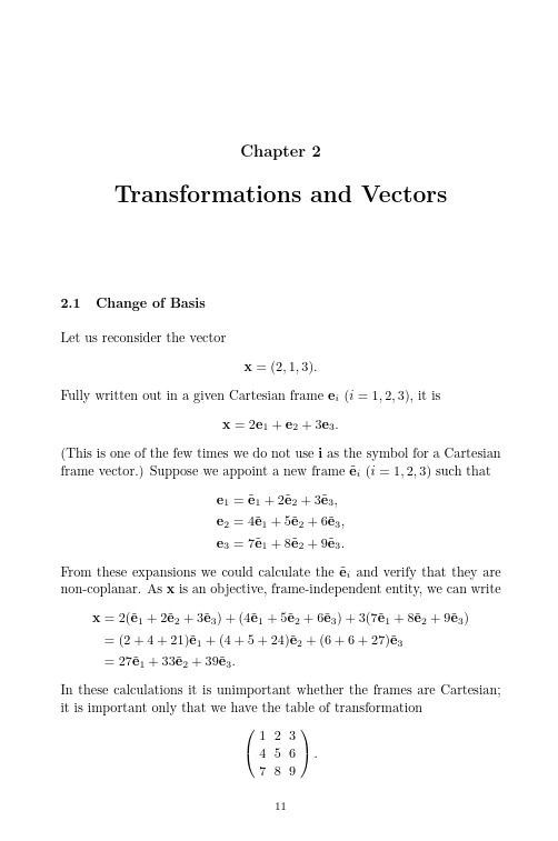
Chapter2Transformations and Vectors2.1Change of BasisLet us reconsider the vectorx=(2,1,3).Fully written out in a given Cartesian frame e i(i=1,2,3),it isx=2e1+e2+3e3.(This is one of the few times we do not use i as the symbol for a Cartesian frame vector.)Suppose we appoint a new frame˜e i(i=1,2,3)such thate1=˜e1+2˜e2+3˜e3,e2=4˜e1+5˜e2+6˜e3,e3=7˜e1+8˜e2+9˜e3.From these expansions we could calculate the˜e i and verify that they are non-coplanar.As x is an objective,frame-independent entity,we can write x=2(˜e1+2˜e2+3˜e3)+(4˜e1+5˜e2+6˜e3)+3(7˜e1+8˜e2+9˜e3)=(2+4+21)˜e1+(4+5+24)˜e2+(6+6+27)˜e3=27˜e1+33˜e2+39˜e3.In these calculations it is unimportant whether the frames are Cartesian; it is important only that we have the table of transformation⎛⎝123 456 789⎞⎠.1112Tensor Analysis with Applications in MechanicsIt is clear that we can repeat the same operation in general form.Let x be of the formx=3i=1x i e i(2.1)with the table of transformation of the frame given ase i=3j=1A ji˜e j.Thenx=3i=1x i3j=1A ji˜e j=3j=1˜e j3i=1A jix i.So in the new basis we havex=3j=1˜x j˜e j where˜x j=3i=1A jix i.Here we have introduced a new notation,placing some indices as subscripts and some as superscripts.Although this practice may seem artificial,there are fairly deep reasons for following it.2.2Dual BasesTo perform operations with a vector x,we must have a straightforward method of calculating its components—ultimately,no matter how ad-vanced we are,we must be able to obtain the x i using simple arithmetic. We prefer formulas that permit us tofind the components of vectors using dot multiplication only;we shall need these when doing frame transfor-mations,etc.In a Cartesian frame the necessary operation is simple dot multiplication by the corresponding basis vector of the frame:we havex k=x·i k(k=1,2,3).This procedure fails in a more general non-Cartesian frame where we do not necessarily have e i·e j=0for all j=i.However,it may still be possible tofind a vector e i such thatx i=x·e i(i=1,2,3)Transformations and Vectors 13in this more general situation.If we set x i =x ·e i =⎛⎝3 j =1x j e j ⎞⎠·e i =3 j =1x j (e j ·e i )and compare the left-and right-hand sides,we see that equality holds whene j ·e i =δi j (2.2)whereδi j = 1,j =i,0,j =i,is the Kronecker delta symbol.In a Cartesian frame we havee k =e k =i kfor each k .Exercise 2.1.Show that e i is determined uniquely by the requirement that x i =x ·e i for every x .Now let us discuss the geometrical nature of the vectors e i .Consider,for example,the equations for e 1:e 1·e 1=1,e 2·e 1=0,e 3·e 1=0.We see that e 1is orthogonal to both e 2and e 3,and its magnitude is such that e 1·e 1=1.Similar properties hold for e 2and e 3.Exercise 2.2.Show that the vectors e i are linearly independent.By Exercise 2.2,the e i constitute a frame or basis.This basis is said to be reciprocal or dual to the basis e i .We can therefore expand an arbitrary vector x asx =3i =1x i e i .(2.3)Note that superscripts and subscripts continue to appear in our notation,but in a way complementary to that used in equation (2.1).If we dot-multiply the representation (2.3)of x by e j and use (2.2)we get x j .This explains why the frames e i and e i are dual:the formulasx ·e i =x i ,x ·e i =x i ,14Tensor Analysis with Applications in Mechanicslook quite similar.So the introduction of a reciprocal basis gives many potential advantages.Let us discuss the reciprocal basis in more detail.Thefirst problem is tofind suitable formulas to define it.We derive these formulas next, butfirst let us note the following.The use of reciprocal vectors may not be practical in those situations where we are working with only two or three vectors.The real advantages come when we are working intensively with many vectors.This is reminiscent of the solution of a set of linear simultaneous equations:it is inefficient tofind the inverse matrix of the system if we have only one forcing vector.But when we must solve such a problem repeatedly for many forcing vectors,the calculation and use of the inverse matrix is reasonable.Writing out x in the e i and e i bases,we used a combination of indices (i.e.,subscripts and superscripts)and summation symbols.From now on we shall omit the symbol of summation when we meet matching subscripts and superscripts:we shall write,say,x i a i.x i a i for the sumiThat is,whenever we see i as a subscript and a superscript,we shall under-stand that a summation is to be carried out over i.This rule shall apply to situations involving vectors as well:we shall understand,for example,x i e i.x i e i to mean the summationiThis rule is called the rule of summation over repeated indices.1Note that a repeated index is a dummy index in the sense that it may be replaced by any other index not already in use:we havex i a i=x1a1+x2a2+x3a3=x k a kfor instance.An index that occurs just once in an expression,for example the index i inA k i x k,is called a free index.In tensor discussions each free index is understood to range independently over a set of values—presently this set is{1,2,3}. 1The rule of summation wasfirst introduced not by mathematicians but by Einstein, and is sometimes referred to as the Einstein summation convention.In a paper where he introduced this rule,Einstein used Cartesian frames and therefore did not distinguish superscripts from subscripts.However,we shall continue to make the distinction so that we can deal with non-Cartesian frames.Transformations and Vectors15 Let us return to the task of deriving formulas for the reciprocal basis vectors e i in terms of the original basis vectors e i.We construct e1first. Since the cross product of two vectors is perpendicular to both,we can satisfy the conditionse2·e1=0,e3·e1=0,by settinge1=c1(e2×e3)where c1is a constant.To determine c1we requiree1·e1=1.We obtainc1[e1·(e2×e3)]=1.The quantity e1·(e2×e3)is a scalar whose absolute value is the volume of the parallelepiped described by the vectors e i.Denoting it by V,we havee1=1V(e2×e3).Similarly,e2=1V(e3×e1),e3=1V(e1×e2).The reader may verify that these expressions satisfy(2.2).Let us mention that if we construct the reciprocal basis to the basis e i we obtain the initial basis e i.Hence we immediately get the dual formulase1=1V(e2×e3),e2=1V(e3×e1),e3=1V(e1×e2),whereV =e1·(e2×e3).Within an algebraic sign,V is the volume of the parallelepiped described by the vectors e i.Exercise2.3.Show that V =1/V.Let us now consider the forms of the dot product between two vectorsa=a i e i=a j e j,b=b p e p=b q e q.16Tensor Analysis with Applications in MechanicsWe havea·b=a i e i·b p e p=a i b p e i·e p.Introducing the notationg ip=e i·e p,(2.4) we havea·b=a i b p g ip.(As a short exercise the reader should write out this expression in full.) Using the reciprocal component representations we geta·b=a j e j·b q e q=a j b q g jqwhereg jq=e j·e q.(2.5) Finally,using a mixed representation we geta·b=a i e i·b q e q=a i b qδq i=a i b iand,similarly,a·b=a j b j.Hencea·b=a i b j g ij=a i b j g ij=a i b i=a i b i.We see that when we use mixed bases to represent a and b we get formulas that resemble the equationa·b=a1b1+a2b2+a3b3from§1.3;otherwise we get more terms and additional multipliers.We will encounter g ij and g ij often.They are the components of a unique tensor known as the metric tensor.In Cartesian frames we obviously haveg ij=δj,g ij=δi j.iTransformations and Vectors17 2.3Transformation to the Reciprocal FrameHow do the components of a vector x transform when we change to the reciprocal frame?We simply setx i e i=x i e iand dot both sides with e j to getx i e i·e j=x i e i·e jorx j=x i g ij.(2.6) In the system of equations⎛⎝x1x2x3⎞⎠=⎛⎝g11g21g31g12g22g32g13g23g33⎞⎠⎛⎝x1x2x3⎞⎠the matrix of the components of the metric tensor g ij is also called the Gram matrix.A theorem in linear algebra states that its determinant is not zero if and only if the vectors e i are linearly independent.Exercise2.4.(a)Show that if the Gram determinant vanishes,then the e i are linearly dependent.(b)Prove that the Gram determinant equals V2.We called the basis e i dual to the basis e i.In e i the metric components are given by g ij,so we can immediately write an expression dual to(2.6):x i=x j g ij.(2.7)We see from(2.6)and(2.7)that,using the components of the metric tensor, we can always change subscripts to superscripts and vice versa.These actions are known as the raising and lowering of indices.Finally,(2.6)and (2.7)together implyx i=g ij g jk x k,henceg ij g jk=δk i.Of course,this means that the matrices of g ij and g ij are mutually inverse.18Tensor Analysis with Applications in MechanicsQuick summaryGiven a basis e i,the vectors e i given by the requirement thate j·e i=δi jare linearly independent and form a basis called the reciprocal or dual basis. The definition of dual basis is motivated by the equation x i=x·e i.The e i can be written ase i=1V(e j×e k)where the ordered triple(i,j,k)equals(1,2,3)or one of the cyclic permu-tations(2,3,1)or(3,1,2),and whereV=e1·(e2×e3).The dual of the basis e k(i.e.,the dual of the dual)is the original basis e k.A given vector x can be expressed asx=x i e i=x i e iwhere the x i are the components of x with respect to the dual basis. Exercise2.5.(a)Let x=x k e k=x k e k.Write out the modulus of x in all possible forms using the metric tensor.(b)Write out all forms of the dot product x·y.2.4Transformation Between General FramesHaving transformed the components x i of a vector x to the corresponding components x i relative to the reciprocal basis,we are now ready to take on the more general task of transforming the x i to the corresponding compo-nents˜x i relative to any other basis˜e i.Let the new basis˜e i be related to the original basis e i bye i=A ji˜e j.(2.8) This is,of course,compact notation for the system of equations⎛⎝e1e2e3⎞⎠=⎛⎝A11A21A31A12A22A32A13A23A33⎞⎠≡A,say⎛⎝˜e1˜e2˜e3⎞⎠.Transformations and Vectors19the subscript indexes Before proceeding,we note that in the symbol A jithe row number in the matrix A,while the superscript indexes the column number.Throughout our development we shall often take the time to write various equations of interest in matrix notation.It follows from(2.8)that=e i·˜e j.A jiExercise2.6.A Cartesian frame is rotated about its third axis to give a new Cartesian frame.Find the matrix of transformation.A vector x can be expressed in the two formsx=x k e k,x=˜x i˜e i.Equating these two expressions for the same vector x,we have˜x i˜e i=x k e k,hence˜e j.(2.9)˜x i˜e i=x k A jkTofind˜x i in terms of x i,we may expand the notation and write(2.9)as ˜x1˜e1+˜x2˜e2+˜x3˜e3=x1A j1˜e j+x2A j2˜e j+x3A j3˜e jwhere,of course,A j1˜e j=A11˜e1+A21˜e2+A31˜e3,A j2˜e j=A12˜e1+A22˜e2+A32˜e3,A j3˜e j=A13˜e1+A23˜e2+A33˜e3.Matching coefficients of the˜e i wefind˜x1=x1A11+x2A12+x3A13=x j A1j,˜x2=x1A21+x2A22+x3A23=x j A2j,˜x3=x1A31+x2A32+x3A33=x j A3j,hence˜x i=x j A i j.(2.10) It is possible to obtain(2.10)from(2.9)in a succinct manner.On the right-hand side of(2.9)the index j is a dummy index which we can replace with20Tensor Analysis with Applications in Mechanicsi and thereby obtain(2.10)immediately.The matrix notation equivalent of(2.10)is⎛⎝˜x1˜x2˜x3⎞⎠=⎛⎝A11A12A13A21A22A23A31A32A33⎞⎠⎛⎝x1x2x3⎞⎠and thus involves multiplication by A T,the transpose of A.We shall also need the equations of transformation from the frame˜e i back to the frame e i.Since the direct transformation is linear the inverse must be linear as well,so we can write˜e i=˜A jie j(2.11) where˜A ji=˜e i·e j.Let usfind the relation between the matrices of transformation A and˜A. By(2.11)and(2.8)we have˜e i=˜A ji e j=˜A jiA k j˜e k,and since the˜e i form a basis we must have˜A jiA k j=δk i. The relationshipA ji ˜A kj=δk ifollows similarly.The product of the matrices(˜A ji)and(A k j)is the unit matrix and thus these matrices are mutually inverse.Exercise2.7.Show that x i=˜x k˜A ik.Formulas for the relations between reciprocal bases can be obtained as follows.We begin with the obvious identitiese j(e j·x)=x,˜e j(˜e j·x)=x.Putting x=˜e i in thefirst of these gives˜e i=A i j e j,while the second identity with x=e i yieldse i=˜A i j˜e j.From these follow the transformation formulas˜x i=x k˜A k i,x i=˜x k A k i.2.5Covariant and Contravariant ComponentsWe have seen that if the basis vectors transform according to the relatione i=A ji˜e j,then the components x i of a vector x must transform according tox i=A ji˜x j.The similarity in form between these two relations results in the x i being termed the covariant components of the vector x.On the other hand,the transformation lawx i=˜A i j˜x jshows that the x i transform like the e i.For this reason the x i are termed the contravariant components of x.We shallfind a further use for this nomenclature in Chapter3.Quick summaryIf frame transformationse i=A ji˜e j,˜e i=˜A ji e j,e i=˜A i j˜e j,˜e i=A ije j,are considered,then x has the various expressionsx=x i e i=x i e i=˜x i˜e i=˜x i˜e i and the transformation lawsx i=A ji˜x j,˜x i=˜A ji x j,x i=˜A i j˜x j,˜x i=A i j x j,apply.The x i are termed contravariant components of x,while the x i are termed covariant components.The transformation laws are particularly simple when the frame is changed to the dual frame.Thenx i=g ji x j,x i=g ij x j,whereg ij=e i·e j,g ij=e i·e j,are components of the metric tensor.2.6The Cross Product in Index NotationIn mechanics a major role is played by the quantity called torque.This quantity is introduced in elementary physics as the product of a force mag-nitude and a length(“force times moment arm”),along with some rules for algebraic sign to account for the sense of rotation that the force would encourage when applied to a physical body.In more advanced discussions in which three-dimensional problems are considered,torque is regarded as a vectorial quantity.If a force f acts at a point which is located relative to an origin O by position vector r,then the associated torque t about O is normal to the plane of the vectors r and f.Of the two possible unit normals,t is conventionally(but arbitrarily)associated with the vectorˆn given by the familiar right-hand rule:if the forefinger of the right hand is directed along r and the middlefinger is directed along f,then the thumb indicates the direction ofˆn and hence the direction of t.The magnitude of t equals|f||r|sinθ,whereθis the smaller angle between f and r.These rules are all encapsulated in the brief symbolismt=r×f.The definition of torque can be taken as a model for a more general operation between vectors:the cross product.If a and b are any two vectors,we definea×b=ˆn|a||b|sinθwhereˆn andθare defined as in the case of torque above.Like any other vector,c=a×b can be expanded in terms of a basis;we choose the reciprocal basis e i and writec=c i e i.Because the magnitudes of a and b enter into a×b in multiplicative fashion, we are prompted to seek c i in the formc i= ijk a j b k.(2.12) Here the ’s are formal coefficients.Let usfind them.We writea=a j e j,b=b k e k,and employ the well-known distributive property(u+v)×w≡u×w+v×wto obtainc =a j e j ×b k e k =a j b k (e j ×e k ).Thenc ·e i =c m e m ·e i =c i =a j b k [(e j ×e k )·e i ]and comparison with (2.12)shows thatijk =(e j ×e k )·e i .Now the value of (e j ×e k )·e i depends on the values of the indices i,j,k .Here it is convenient to introduce the idea of a permutation of the ordered triple (1,2,3).A permutation of (1,2,3)is called even if it can be brought about by performing any even number of interchanges of pairs of these numbers;a permutation is odd if it results from performing any odd number of interchanges.We saw before that (e j ×e k )·e i equals the volume of the frame parallelepiped if i,j,k are distinct and the ordered triple (i,j,k )is an even permutation of (1,2,3).If i,j,k are distinct and the ordered triple (i,j,k )is an odd permutation of (1,2,3),we obtain minus the volume of the frame parallelepiped.If any two of the numbers i,j,k are equal we obtain zero.Hence ijk =⎧⎪⎪⎨⎪⎪⎩+V,(i,j,k )an even permutation of (1,2,3),−V,(i,j,k )an odd permutation of (1,2,3),0,two or more indices equal.Moreover,it can be shown (Exercise 2.4)thatV 2=gwhere g is the determinant of the matrix formed from the elements g ij =e i ·e j of the metric tensor.Note that |V |=1for a Cartesian frame.The permutation symbol ijk is useful in writing formulas.For example,the determinant of a matrix A =(a ij )can be expressed succinctly asdet A = ijk a 1i a 2j a 3k .Much more than a notational device however, ijk represents a tensor (the so-called Levi–Civita tensor ).We discuss this further in Chapter 3.Exercise 2.8.The contravariant components of a vector c =a ×b can be expressed asc i = ijk a j b kfor suitable coefficients ijk .Use the technique of this section to find the coefficients.Then establish the identity ijk pqr = δp i δq i δr i δp j δq j δr j δp k δq kδr k and use it to show thatijk pqk =δp i δq j −δq i δp j .Use this in turn to prove thata ×(b ×c )=b (a ·c )−c (a ·b )(2.13)for any vectors a ,b ,c .Exercise 2.9.Establish Lagrange’s identity(a ×b )·(c ×d )=(a ·c )(b ·d )−(a ·d )(b ·c ).2.7Norms on the Space of Vectors We often need to characterize the intensity of some vector field locally or globally.For this,the notion of a norm is appropriate.The well-known Euclidean norm of a vector a =a k i k written in a Cartesian frame isa = 3 k =1a 2k1/2.This norm is related to the inner product of two vectors a =a k i k and b =b k i k :we have a ·b =a k b k so thata =(a ·a )1/2.In a non-Cartesian frame,the components of a vector depend on the lengths of the frame vectors and the angles between them.Since the sum of squared components of a vector depends on the frame,we cannot use it to characterize the vector.But the formulas connected with the dot product are invariant under change of frame,so we can use them to characterize the intensity of the vector —its length.Thus for two vectors x =x i e i and y =y j e j written in the arbitrary frame,we can introduce a scalar product (i.e.,a simple dot product)x ·y =x i e i ·y j e j =x i y j g ij =x i y j g ij =x i y i .Note that only in mixed coordinates does this resemble the scalar product in a Cartesian frame.Similarly,the norm of a vector x isx =(x·x)1/2=x i x j g ij1/2=x i x j g ij1/2=x i x i1/2.This dot product and associated norm have all the properties required from objects of this nature in algebra or functional analysis.Indeed,it is neces-sary only to check whether all the axioms of the inner product are satisfied.(i)x·x≥0,and x·x=0if and only if x=0.This property holdsbecause all the quantities involved can be written in a Cartesianframe where it holds trivially.By the same reasoning,we confirmsatisfaction of the property(ii)x·y=y·x.The reader should check that this holds for any representation of the vectors.Finally,(iii)(αx+βy)·z=α(x·z)+β(y·z)whereαandβare arbitrary real numbers and z is a vector.By the general theory then,the expressionx =(x·x)1/2(2.14) satisfies all the axioms of a norm:(i) x ≥0,with x =0if and only if x=0.(ii) αx =|α| x for any realα.(iii) x+y ≤ x + y .In addition we have the Schwarz inequalityx·y ≤ x y ,(2.15) where in the case of nonzero vectors the equality holds if and only if x=λy for some realλ.The set of all three-dimensional vectors constitutes a three-dimensional linear space.A linear space equipped with the norm(2.14)becomes a normed space.In this book,the principal space is R3.Note that we can introduce more than one norm in any normed space,and in practice a variety of norms turn out to be necessary.For example,2 x is also a norm in R3.We can introduce other norms,quite different from the above. One norm can be introduced as follows.Let e k be a basis of R3and letx =x k e k .For p ≥1,we introduce x p =3 k =1|x k |p 1/p.Norm axioms (i)and (ii)obviously hold.Axiom (iii)is a consequence of the classical Minkowski inequality for finite sums.The reader should be aware that this norm is given in a certain basis.If we use it in another basis,the value of the norm of a vector will change in general.An advantage of the norm (2.14)is that it is independent of the basis of the space.Later,when investigating the eigenvalues of a tensor,we will need a space of vectors with complex components.It can be introduced similarly to the space of complex numbers.We start with the space R 3having basis e k ,and introduce multiplication of vectors in R 3by complex numbers.This also yields a linear space,but it is complex and denoted by C 3.An arbitrary vector x in C 3takes the formx =(a k +ib k )e k ,where i is the imaginary unit (i 2=−1).Analogous to the conjugate number is the conjugate vector to x ,defined byx =(a k −ib k )e k .The real and imaginary parts of x are a k e k and b k e k ,respectively.Clearly,a basis in C 3may contain vectors that are not in R 3.As an exercise,the reader should write out the form of the real and imaginary parts of x in such a basis.In C 3,the dot product loses the property that x ·x ≥0.However,we can introduce the inner product of two vectors x and y asx ,y =x ·y .It is easy to see that this inner product has the following properties.Let x ,y ,z be arbitrary vectors of C 3.Then(i)x ·x ≥0,and x ·x =0if and only if x =0.(ii)x ·y =y ·x .(iii)(αx +βy )·z =α(x ·z )+β(y ·z )where αand βare arbitrarycomplex numbers.The reader should verify these properties.Now we can introduce the norm related to the inner product,x = x ,x 1/2,and verify that it satisfies all the axioms of a norm in a complex linear space.As a consequence of the general properties of the inner product, Schwarz’s inequality(2.15)also holds in C3.2.8Closing RemarksWe close by repeating something we said in Chapter1:A vector is an objective entity.In elementary mathematics we learn to think of a vector as an ordered triple of components.There is,of course,no harm in this if we keep in mind a certain Cartesian frame.But if wefix those components then in any other frame the vector is determined uniquely.Absolutely uniquely!So a vector is something objective,but as soon as we specify its components in one frame we canfind them in any other frame by the use of certain rules.We emphasize this because the situation is exactly the same with ten-sors.A tensor is an objective entity,andfixing its components relative to one frame,we determine the tensor uniquely—even though its components relative to other frames will in general be different.2.9Problems2.1Find the dual basis to e i.(a)e1=2i1+i2−i3,e2=2i2+3i3,e3=i1+i3;(b)e1=i1+3i2+2i3,e2=2i1−3i2+2i3,e3=3i1+2i2+3i3;(c)e1=i1+i2,e2=i1−i2,e3=3i3;(d)e1=cosφi1+sinφi2,e2=−sinφi1+cosφi2,e3=i3.2.2Let˜e1=−2i1+3i2+2i3,e1=2i1+i2−i3,˜e2=−2i1+2i2+i3,e2=2i2+3i3,˜e3=−i1+i2+i3,e3=i1+i3.Find the matrix A jof transformation from the basis˜e i to the basis e j.i2.3Let˜e1=i1+2i2,e1=i1−6i3,˜e2=−i2−i3,e2=−3i1−4i2+4i3,˜e3=−i1+2i2−2i3,e3=i1+i2+i3. Find the matrix of transformation of the basis˜e i to e j.2.4Find(a)a jδjk,(b)a i a jδi j,(c)δi i,(d)δijδjk,(e)δijδji,(f)δji δk jδik.2.5Show that ijk ijl=2δlk.2.6Show that ijk ijk=6.2.7Find(a) ijkδjk,(b) ijk mkjδi m,(c) ijkδk mδj n,(d) ijk a i a j,(e) ijk| ijk|,(f) ijk imnδj m.2.8Find(a×b)×c.2.9Show that(a×b)·a=0.2.10Show that a·(b×c)d=(a·d)b×c+(b·d)c×a+(c·d)a×b.2.11Show that(e×a)×e=a if|e|=1and e·a=0.2.12Let e k be a basis of R3,let x=x k e k,and suppose h1,h2,h3arefixed positive numbers.Show that h k|x k|is a norm in R3.。
(完整版)张量分析中文翻译
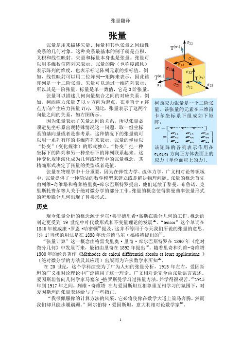
张量张量是用来描述矢量、标量和其他张量之间线性关系的几何对象。
这种关系最基本的例子就是点积、叉积和线性映射。
矢量和标量本身也是张量。
张量可以用多维数值阵列来表示。
张量的阶(也称度或秩)表示阵列的维度,也表示标记阵列元素的指标值。
例如,线性映射可以用二位阵列--矩阵来表示,因此该阵列是一个二阶张量。
矢量可以通过一维阵列表示,所以其是一阶张量。
标量是单一数值,它是0阶张量。
张量可以描述几何向量集合之间的对应关系。
例如,柯西应力张量T 以v 方向为起点,在垂直于v 终点方向产生应力张量T(v),因此,张量表示了这两个 向量之间的关系,如右图所示。
因为张量表示了矢量之间的关系,所以张量必 须避免坐标系出现特殊情况这一问题。
取一组坐标 系的基向量或者是参考系,这种情况下的张量就可 以用一系列有序的多维阵列来表示。
张量的坐标以 “协变”(变化规律)的形式独立,“协变”把一种 坐标下的阵列和另一种坐标下的阵列联系起来。
这 种变化规律演化成为几何或物理中的张量概念,其 精确形式决定了张量的类型或者是值。
张量在物理学中十分重要,因为在弹性力学、流体力学、广义相对论等领域中,张量提供了一种简洁的数学模型来建立或是解决物理问题。
张量的概念首先由列维-奇维塔和格莱格里奥-库尔巴斯特罗提出,他们延续了黎曼、布鲁诺、克里斯托费尔等人关于绝对微分学的部分工作。
张量的概念使得黎曼曲率张量形式的流形微分几何出现了替换形式。
历史现今张量分析的概念源于卡尔•弗里德里希•高斯在微分几何的工作,概念的制定更受到19世纪中叶代数形式和不变量理论的发展[2]。
“tensor ”这个单词在1846年被威廉·罗恩·哈密顿[3]提及,这并不等同于今天我们所说的张量的意思。
[注1]当代的用法是在1898年沃尔德马尔·福格特提出的[4]。
“张量计算”这一概念由格雷戈里奥·里奇·库尔巴斯特罗在1890年《绝对微分几何》中发展而来,最初由里奇在1892年提出[5]。
学习张量必看一个文档学会张量张量分析

Appendix A.1
张量基本概念
➢ 指标符号使用方法
1. 三维空间中任意点 P 旳坐标(x, y, z)可缩写成 xi , 其中x1=x, x2=y, x3=z。
2. 两个矢量 a 和 b 旳分量旳点积(或称数量积)为:
3
a b= a1b1 a2b2 a3b3 aibi i 1
3. 换标符号,具有换标作用。例如:
d s2 ij d xi d x j d xi d xi d x j d x j
即:假如符号 旳两个指标中,有一种和同项中其他
因子旳指标相重,则能够把该因子旳那个重指标换成
旳另一种指标,而 自动消失。
30
符号ij 与erst
类似地有
ij a jk aik ; ij aik a jk ij akj aki ; ij aki akj ij jk ik ; ij jkkl il
ij
1 0
(i = j) (i, j=1, 2, …, n) (i j)
➢ 特征
1. 对称性,由定义可知指标 i 和 j 是对称旳,即
ij ji
29
符号ij 与erst
2. ij 旳分量集合相应于单位矩阵。例如在三维空间
11 12 13 1 0 0
21
22
23
0
1
0
31 32 33 0 0 1
27
目录
引言 张量旳基本概念,爱因斯坦求和约定
符号ij与erst
坐标与坐标转换 张量旳分量转换规律,张量方程 张量代数,商法则 常用特殊张量,主方向与主分量 张量函数及其微积分
Appendix A
28
符号ij 与erst
➢ ij 符号 (Kronecker delta)
Introduction to Tensor Calculus and Continuum Mechanics 张量分析 英文版 part1
Introduction toTensor CalculusandContinuum Mechanicsby J.H.HeinbockelDepartment of Mathematics and StatisticsOld Dominion UniversityPREF ACEThis is an introductory text which presents fundamental concepts from the subject areas of tensor calculus,differential geometry and continuum mechanics.The material presented is suitable for a two semester course in applied mathematics and isflexible enough to be presented to either upper level undergraduate or beginning graduate students majoring in applied mathematics,engineering or physics.The presentation assumes the students have some knowledge from the areas of matrix theory,linear algebra and advanced calculus.Each section includes many illustrative worked examples.At the end of each section there is a large collection of exercises which range in difficulty.Many new ideas are presented in the exercises and so the students should be encouraged to read all the exercises.The purpose of preparing these notes is to condense into an introductory text the basic definitions and techniques arising in tensor calculus,differential geometry and continuum mechanics.In particular,the material is presented to(i)develop a physical understanding of the mathematical concepts associated with tensor calculus and(ii)develop the basic equations of tensor calculus,differential geometry and continuum mechanics which arise in engineering applications.From these basic equations one can go on to develop more sophisticated models of applied mathematics.The material is presented in an informal manner and uses mathematics which minimizes excessive formalism.The material has been divided into two parts.Thefirst part deals with an introduc-tion to tensor calculus and differential geometry which covers such things as the indicial notation,tensor algebra,covariant differentiation,dual tensors,bilinear and multilinear forms,special tensors,the Riemann Christoffel tensor,space curves,surface curves,cur-vature and fundamental quadratic forms.The second part emphasizes the application of tensor algebra and calculus to a wide variety of applied areas from engineering and physics. The selected applications are from the areas of dynamics,elasticity,fluids and electromag-netic theory.The continuum mechanics portion focuses on an introduction of the basic concepts from linear elasticity andfluids.The Appendix A contains units of measurements from the Syst`e me International d’Unit`e s along with some selected physical constants.The Appendix B contains a listing of Christoffel symbols of the second kind associated with various coordinate systems.The Appendix C is a summary of useful vector identities.J.H.Heinbockel,1996Copyright c 1996by J.H.Heinbockel.All rights reserved.Reproduction and distribution of these notes is allowable provided it is for non-profit purposes only.INTRODUCTION TOTENSOR CALCULUSANDCONTINUUM MECHANICSPART1:INTRODUCTION TO TENSOR CALCULUS§1.1INDEX NOTATION (1)Exercise1.1 (28)§1.2TENSOR CONCEPTS AND TRANSFORMATIONS (35)Exercise1.2 (54)§1.3SPECIAL TENSORS (65)Exercise1.3 (101)§1.4DERIV ATIVE OF A TENSOR (108)Exercise1.4 (123)§1.5DIFFERENTIAL GEOMETRY AND RELATIVITY (129)Exercise1.5 (162)PART2:INTRODUCTION TO CONTINUUM MECHANICS§2.1TENSOR NOTATION FOR VECTOR QUANTITIES (171)Exercise2.1 (182)§2.2DYNAMICS (187)Exercise2.2 (206)§2.3BASIC EQUATIONS OF CONTINUUM MECHANICS (211)Exercise2.3 (238)§2.4CONTINUUM MECHANICS(SOLIDS) (243)Exercise2.4 (272)§2.5CONTINUUM MECHANICS(FLUIDS) (282)Exercise2.5 (317)§2.6ELECTRIC AND MAGNETIC FIELDS (325)Exercise2.6 (347)BIBLIOGRAPHY (352)APPENDIX A UNITS OF MEASUREMENT (353)APPENDIX B CHRISTOFFEL SYMBOLS OF SECOND KIND355 APPENDIX C VECTOR IDENTITIES (362)INDEX (363)。
张量分解与MATLAB Tensor Toolbox
Observe: For two vectors a and b, a ◦ b and a ⊗ b have the same elements, but one is shaped into a matrix and the other into a vector.
Tamara G. Kolda – UMN – April 27, 2007 - p.7
Proposed by Tucker (1966) AKA: Three-mode factor analysis, three-mode PCA, orthogonal array decomposition A, B, and C may be orthonormal (generally assume they have full column rank) G is not diagonal Not unique
Tamara G. Kolda – UMN – April 27, 2007 - p.2
A tensor is a multidimensional array
An I × J × K tensor
K
Column (Mode-1) Fibers
Row (Mode-2) Fibers
Tube (Mode-3) Fibers
to from
authority scores for 2nd topic
hub scores for 1st topic
Jon M. Kleinberg. Authoritative sources in a hyperlinked environment. J. ACM, 46(5):604–632, 1999. (doi:10.1145/324133.324140)
Gradient Shrinking Solitons with Vanishing Weyl Tensor
further that, it has nonnegative Ricci curvature and the growth of the Riemannian curvature is not faster that ea(r(x)+1) , where r (x) is the distance function and a is a suitable positive constant, then its universal cover is either Rn , S n , or S n−1 × R. This result had been improved by Peterson-Wylie (Theorem 1.2 and the remark 1.3 of [17]) in which they only need to assume the Ricci curvature is bounded from 2 2 below and the growth of the Ricci curvature is not faster than e 5 cr(x) outside of a compact set, where c < λ . We also notice that Cao-Wang [2] had an alternative 2 proof of the Ni-Wallach’s result [15]. The key point to get the above complete classification theorem on 3-dimensional complete gradient shrinking soliton without curvature bound assumption is the local version of the Hamilton-Ivey pinching estimate. The Hamilton-Ivey pinching estimate in 3-dimension plays a crucial role in the analysis of the Ricci flow. An open question is how to generalize Hamilton-Ivey’s to high dimension. In [20], the author obtained the following (global) Hamilton-Ivey type pinching estimate on high dimension: Suppose we have a solution to the Ricci flow on a n-dimension manifold which is complete with bounded curvature and vanishing Weyl tensor for each t ≥ 0. Assume at t = 0 the least eigenvalue of the curvature operator at each point are bounded below by ν ≥ −1. Then at all points and all times t ≥ 0 we have the pinching estimate n(n + 1) ] 2 whenever ν < 0. In the present paper, we will get a local version of this HamiltonIvey type pinching estimate for the gradient shrinking solitons with vanishing Weyl tensor (without curvature bound). Based on this pinching estimate, we will obtain the following complete classification theorem (without any curvature bound assumption): R ≥ (−ν )[log(−ν ) + log(1 + t) − Theorem 1.2 Any complete gradient shrinking soliton with vanishing Weyl tensor must be the finite quotients of Rn , S n−1 × R, or S n . This paper contains three sections and the organization is as follows. In section 2, we will prove an algebra lemma which will be used to prove the local version of the Hamilton-Ivey type pinching estimate. In section 3, we will give some propositions and finish the proof of the theorem 1.2. Acknowledgement I would be indebted to my advisor Professor X.P.Zhu for provoking the interest to this problem and many suggestions and discussions. 3
Decay Constants $f_{D_s^}$ and $f_{D_s}$ from ${bar{B}}^0to D^+ l^- {bar{nu}}$ and ${bar{B}
form factor.
PACS index : 12.15.-y, 13.20.-v, 13.25.Hw, 14.40.Nd, 14.65.Fy Keywards : Factorization, Non-leptonic Decays, Decay Constant, Penguin Effects
∗ experimentally from leptonic B and Ds decays. For instance, determine fB , fBs fDs and fDs
+ the decay rate for Ds is given by [1]
+ Γ(Ds
m2 G2 2 2 l 1 − m M → ℓ ν ) = F fD D s 2 8π s ℓ MD s
1/2
(4)
.
(5)
In the zero lepton-mass limit, 0 ≤ q 2 ≤ (mB − mD )2 .
2
For the q 2 dependence of the form factors, Wirbel et al. [8] assumed a simple pole formula for both F1 (q 2 ) and F0 (q 2 ) (we designate this scenario ’pole/pole’): q2 F1 (q ) = F1 (0) /(1 − 2 ), mF1
∗ amount to about 11 % for B → DDs and 5 % for B → DDs , which have been mentioned in
Tensor Permutation Matrices in Finite Dimensions
which has the following properties : for any unicolumns and two rows matrices [α] = α1 α2 β1 ∈ M2×1 (K) β2 [U2⊗2 ]·( [α]⊗[β ] ) = [β ]⊗[α] ∈ M2×1 (K), [β ] = 1
3
1 i2 i3 [M ] = Mji1 j2 j3
[M ] =
1 0 1 1 0 0 0 0 1 1 1 1 4 5 1 6 3 2 1 1 1 1 0 0 3 2 1 7 8 9 9 8 7 6 5 4 3 2
1 0 1 2 3 4 5 6 5 4 3 2 3 4 5 6 9 8 7 6 1 0 1 2
7 8 9 0 9 8 7 6 1 0 1 2 7 8 9 0 5 4 3 2 3 4 5 6
[U3⊗3 ] =
algebra and multilinear algebra [6]. In establishing firstly, the theorems on linear operators in intrinsic way, that is independently of the basis, and after that we demonstrate the analogous theorems for the matrices. Define [Un⊗p ] as the tensor commutation matrix n ⊗ p, n, p ∈ N⋆ , whose elements are 0 or 1. In this article we have given two manners to construct [Un⊗p ] for any n and p ∈ N⋆ , and we have constructed a formula which allows us to construct the tensor permutation matrix [Un1 ⊗n2 ⊗...⊗nk (σ )], ( n1 , n2 , . . ., nk ) ∈ N⋆ and a formula which gives us the expression of their elements. From (1) it is normal to think to what about the expression of [U3⊗3 ] by using Gell-Mann matrices. But at first we are obliged to talk a bit about the definitions of the types of matrices, and after that we are going to expose the properties of tensor product. Define [In ] as the n × n unit matrix. For the vectors and covectors we have used the RAOELINA ANDRIAMBOLOLONA’s notations[7], with overlining for the vectors, x, and underlining for the covectors, ϕ. Throughout this article K = R or C.
张量分析-第10讲LJ
时间 t 求导. Euler 坐标系中求物质导数时, 不仅要考虑物理自身随时间的变化, 而且要考虑由于质点运动而引起的位置坐标 x i 的变化. Lagrange 坐标系一般是曲线坐标系, 而Euler坐标系可以取直角坐 标系,一般在推导时采用Lagrange坐标系, 然后转换到Euler坐标系 中进行计算. 5
ˆi dg ˆ v) g ˆ i ( ˆi E g ˆi ω g dt
ˆi dg ˆ ) g ˆ i ( v ˆ i (E - Ω) g ˆi E g ˆ i Ω g ˆi E g ˆi ω g dt
13
4.3 欧拉坐标系基矢量的物质导数
r r ( x i (t )),
2. Lagrange坐标
r ( x j (t )) j gi g ( x (t )) i i x
ξ3
拉格朗月坐标是嵌在质点上, 随物体一起运动和变形, 又称随体坐标或嵌入坐标: i ξ3 变形前后的同一个质点坐标值不 B g ξ2 改变, 但是两质点的距离在变形前 A 后发生了变化。
ˆij dT
j ˆij d T ˆ ˆ d g dT d ˆ i d g j j i j i ˆ j i g ˆ j g ˆ ig ˆ T ˆ T ˆi ˆ ig ˆ ) (T j g g dt dt dt dt dt
ˆ r ˆ ˆi dr ( i ) t d i d i g ˆ r ˆ ˆ i ( j , t ) g i ( i )t g
ξ3
B A
3 g
ξ3
ˆ3 g
B'
ˆ2 g
A'
- 1、下载文档前请自行甄别文档内容的完整性,平台不提供额外的编辑、内容补充、找答案等附加服务。
- 2、"仅部分预览"的文档,不可在线预览部分如存在完整性等问题,可反馈申请退款(可完整预览的文档不适用该条件!)。
- 3、如文档侵犯您的权益,请联系客服反馈,我们会尽快为您处理(人工客服工作时间:9:00-18:30)。
TensorTensors are geometric objects that describe linearrelations between vectors, scalars, and other tensors.Elementary examples of such relations include thedot product, the cross product, and linearmaps.Vectors and scalars themselves are also tensors.A tensor can be represented as a multi-dimensionalarray of numerical values. The order (also degree orrank )of a tensor is the dimensionality of the arrayneeded to represent it, or equivalently, the number ofindices needed to label a component of that array. For example, a linear map can be represented by a matrix, a 2-dimensional array, and therefore is a 2nd-order tensor. A vector can be represented as a 1-dimensional array and is a1st-order tensor. Scalars are single numbers andare thus 0th-order tensors.Tensors are used to represent correspondences between sets of geometric vectors. For example, the Cauchy stress tensor T takes a direction v as input and produces the stress T (v ) on the surfacenormal to this vector for output thus expressinga relationship between these two vectors, shown in the figure (right).Because they express a relationship between vectors, tensors themselves must beindependent of a particular choice of coordinate system. Taking a coordinate basis or frame of reference and applying the tensor to it results in an organized multidimensional array representing the tensor in that basis, or frame of reference. The coordinate independence of a tensor then takes the form of a "covariant" transformation law that relates the array computed in one coordinate system to that computed in another one. This transformation law is considered to be built into the notion of a tensor in a geometric or physical setting, and the precise form of the transformation law determines the type (or valence ) of the tensor.Tensors are important in physics because they provide a concise mathematical framework for formulating and solving physics problems in areas such as elasticity, fluid mechanics, and general relativity. Tensors were first conceived by Tullio Levi-Civita and Gregorio Ricci-Curbastro, who continued the earlier work of Bernhard Riemann and Elwin Bruno Christoffel and others, as part of the absolute differential calculus . The concept enabled an alternative formulation of the intrinsic differential geometry of a manifold in the form of the Riemann curvature tensor.[1] Cauchy stress tenso r , a second-order tensor. The tensor's components, in a three-dimensional Cartesian coordinate system, form the matrix whose columns are the stresses (forces per unit area) acting on the e 1, e 2, and e 3 faces of the cube.HistoryThe concepts of later tensor analysis arose from the work of Carl Friedrich Gauss in differential geometry, and the formulation was much influenced by the theory of algebraic forms and invariants developed during the middle of the nineteenth century.[2]The word "tensor" itself was introduced in 1846 by William Rowan Hamilton[3] to describe something different from what is now meant by a tensor.[Note 1] The contemporary usage was brought in by Woldemar V oigt in 1898.[4]Tensor calculus was developed around 1890 by Gregorio Ricci-Curbastro under the title absolute differential calculus, and originally presented by Ricci in 1892.[5] It was made accessible to many mathematicians by the publication of Ricci and Tullio Levi-Civita's 1900 classic text Méthodes de calcul différentiel absolu et leurs applications (Methods of absolute differential calculus and their applications).[6]In the 20th century, the subject came to be known as tensor analysis, and achieved broader acceptance with the introduction of Einstein's theory of general relativity, around 1915. General relativity is formulated completely in the language of tensors. Einstein had learned about them, with great difficulty, from the geometer Marcel Grossmann.[7]Levi-Civita then initiated a correspondence with Einstein to correct mistakes Einstein had made in his use of tensor analysis. The correspondence lasted 1915–17, and was characterized by mutual respect:I admire the elegance of your method of computation; it must be nice to ride through these fields upon the horse of true mathematics while the like of us have to make our way laboriously on foot.—Albert Einstein, The Italian Mathematicians of Relativity[8]Tensors were also found to be useful in other fields such as continuum mechanics. Some well-known examples of tensors in differential geometry are quadratic forms such as metric tensors, and the Riemann curvature tensor. The exterior algebra of Hermann Grassmann, from the middle of the nineteenth century, is itself a tensor theory, and highly geometric, but it was some time before it was seen, with the theory of differential forms, as naturally unified with tensor calculus. The work of Élie Cartan made differential forms one of the basic kinds of tensors used in mathematics. From about the 1920s onwards, it was realised that tensors play a basic role in algebraic topology (for example in the Künneth theorem).[citation needed] Correspondingly there are types of tensors at work in many branches of abstract algebra, particularly in homological algebra and representation theory. Multilinear algebra can be developed in greater generality than for scalars coming from a field, but the theory is then certainly less geometric, and computations more technical and less algorithmic.[clarification needed]Tensors are generalized within category theory bymeans of the concept of monoidal category, from the 1960s.DefinitionThere are several approaches to defining tensors. Although seemingly different, the approaches just describe the same geometric concept using different languages and at different levels of abstraction.As multidimensional arraysJust as a scalar is described by a single number, and a vector with respect to a given basis is described by an array of one dimension, any tensor with respect to a basis is described by a multidimensional array. The numbers in the array are known as the scalar components of the tensor or simply its components.They are denoted by indices giving their position in the array, in subscript and superscript, after the symbolic name of the tensor. The total number of indices required to uniquely select each component is equal to the dimension of the array, and is called the order or the rank of the tensor.[Note 2]For example, the entries of an order 2 tensor T would be denoted T ij, where i and j are indices running from 1 to the dimension of the related vector space.[Note 3]Just as the components of a vector change when we change the basis of the vector space, the entries of a tensor also change under such a transformation. Each tensor comes equipped with a transformation law that details how the components of the tensor respond to a change of basis. The components of a vector can respond in two distinct ways to a change of basis (see covariance and contravariance of vectors),where the new basis vectors are expressed in terms of the old basis vectors as,where R i j is a matrix and in the second expression the summation sign was suppressed (a notational convenience introduced by Einstein that will be used throughout this article). The components, v i, of a regular (or column) vector, v, transform with the inverse of the matrix R,where the hat denotes the components in the new basis. While the components, w i, of a covector (or row vector), w transform with the matrix R itself,The components of a tensor transform in a similar manner with a transformation matrix for each index. If an index transforms like a vector with the inverse of the basis transformation, it is called contravariant and is traditionally denoted with an upper index, while an index that transforms with the basis transformation itself is called covariant and is denoted with a lower index. The transformation law for an order-m tensor with n contravariant indices and m−n covariant indices is thus given as,Such a tensor is said to be of order or type (n,m−n).[Note 4] This discussion motivates the following formal definition:[9]Definition. A tensor of type (n, m−n) is an assignment of a multidimensional arrayto each basis f = (e1,...,e N) such that, if we apply the change of basisthen the multidimensional array obeys the transformation lawThe definition of a tensor as a multidimensional array satisfying a transformation law traces back to the work of Ricci.[1]Nowadays, this definition is still used in some physics and engineering text books.[10][11]Tensor fieldsMain article: Tensor fieldIn many applications, especially in differential geometry and physics, it is natural to consider a tensor with components which are functions. This was, in fact, the setting of Ricci's original work. In modern mathematical terminology such an object is called a tensor field, but they are often simply referred to as tensors themselves.[1]In this context the defining transformation law takes a different form. The "basis" for the tensor field is determined by the coordinates of the underlying space, and thedefining transformation law is expressed in terms of partial derivatives of thecoordinate functions, , defining a coordinate transformation,[1]As multilinear mapsA downside to the definition of a tensor using the multidimensional array approach is that it is not apparent from the definition that the defined object is indeed basis independent, as is expected from an intrinsically geometric object. Although it is possible to show that transformation laws indeed ensure independence from the basis, sometimes a more intrinsic definition is preferred. One approach is to define a tensor as a multilinear map. In that approach a type (n,m) tensor T is defined as a map,where V is a vector space and V* is the corresponding dual space of covectors, which is linear in each of its arguments.By applying a multilinear map T of type (n,m) to a basis {e j} for V and a canonical cobasis {εi} for V*,an n+m dimensional array of components can be obtained. A different choice of basis will yield different components. But, because T is linear in all of its arguments, the components satisfy the tensor transformation law used in the multilinear array definition. The multidimensional array of components of T thus form a tensor according to that definition. Moreover, such an array can be realised as the components of some multilinear map T. This motivates viewing multilinear maps as the intrinsic objects underlying tensors.Using tensor productsMain article: Tensor (intrinsic definition)For some mathematical applications, a more abstract approach is sometimes useful. This can be achieved by defining tensors in terms of elements of tensor products of vector spaces, which in turn are defined through a universal property. A type (n,m) tensor is defined in this context as an element of the tensor product of vectorspaces,[12]If v i is a basis of V and w j is a basis of W, then the tensor product has anatural basis . The components of a tensor T are the coefficients of the tensor with respect to the basis obtained from a basis {e i} for V and its dual {εj}, i.e.Using the properties of the tensor product, it can be shown that these components satisfy the transformation law for a type (m,n) tensor. Moreover, the universal property of the tensor product gives a 1-to-1 correspondence between tensors defined in this way and tensors defined as multilinear maps.OperationsThere are a number of basic operations that may be conducted on tensors that again produce a tensor. The linear nature of tensor implies that two tensors of the same type may be added together, and that tensors may be multiplied by a scalar with results analogous to the scaling of a vector. On components, these operations are simply performed component for component. These operations do not change the type of the tensor, however there also exist operations that change the type of the tensors.Raising or lowering an indexMain article: Raising and lowering indicesWhen a vector space is equipped with an inner product (or metric as it is often called in this context), operations can be defined that convert a contravariant (upper) index into a covariant (lower) index and vice versa. A metric itself is a (symmetric) (0,2)-tensor, it is thus possible to contract an upper index of a tensor with one of lower indices of the metric. This produces a new tensor with the same index structure as the previous, but with lower index in the position of the contracted upper index. This operation is quite graphically known as lowering an index.Conversely the matrix inverse of the metric can be defined, which behaves as a (2,0)-tensor. This inverse metric can be contracted with a lower index to produce an upper index. This operation is called raising an index.ApplicationsContinuum mechanicsImportant examples are provided by continuum mechanics. The stresses inside a solid body or fluid are described by a tensor. The stress tensor and strain tensor are both second order tensors, and are related in a general linear elastic material by a fourth-order elasticity tensor. In detail, the tensor quantifying stress in a 3-dimensional solid object has components that can be conveniently represented as a 3×3 array. The three faces of a cube-shaped infinitesimal volume segment of the solid are each subject to some given force. The force's vector components are also three in number. Thus, 3×3, or 9 components are required to describe the stress at this cube-shaped infinitesimal segment. Within the bounds of this solid is a whole mass of varying stress quantities, each requiring 9 quantities to describe. Thus, a second order tensor is needed.If a particular surface element inside the material is singled out, the material on one side of the surface will apply a force on the other side. In general, this force will not be orthogonal to the surface, but it will depend on the orientation of the surface in a linear manner. This is described by a tensor of type (2,0), in linear elasticity, or more precisely by a tensor field of type (2,0), since the stresses may vary from point to point.Other examples from physicsCommon applications include∙Electromagnetic tensor(or Faraday's tensor) in electromagnetism∙Finite deformation tensors for describing deformations and strain tensor for strain in continuum mechanics∙Permittivity and electric susceptibility are tensors in anisotropic media∙Four-tensorsin general relativity (e.g. stress-energy tensor), used to represent momentum fluxes∙Spherical tensor operators are the eigen functions of the quantum angular momentum operator in spherical coordinates∙Diffusion tensors, the basis of Diffusion Tensor Imaging, represent rates of diffusion in biologic environments∙Quantum Mechanicsand Quantum Computing utilise tensor products for combination of quantum statesApplications of tensors of order > 2The concept of a tensor of order two is often conflated with that of a matrix. Tensors of higher order do however capture ideas important in science and engineering, as has been shown successively in numerous areas as they develop. This happens, for instance, in the field of computer vision, with the trifocal tensor generalizing the fundamental matrix.The field of nonlinear optics studies the changes to material polarization density underextreme electric fields. The polarization waves generated are related to the generating electric fields through the nonlinear susceptibility tensor. If the polarization P is not linearly proportional to the electric field E, the medium is termed nonlinear. To a good approximation (for sufficiently weak fields, assuming no permanent dipole moments are present), P is given by a Taylor series in E whose coefficients are the nonlinear susceptibilities:Here is the linear susceptibility, gives the Pockels effect and secondharmonic generation, and gives the Kerr effect. This expansion shows the way higher-order tensors arise naturally in the subject matter.Generalizations[edit]Tensors in infinite dimensionsThe notion of a tensor can be generalized in a variety of ways to infinite dimensions. One, for instance, is via the tensor product of Hilbert spaces.[15]Another way of generalizing the idea of tensor, common in nonlinear analysis, is via the multilinear maps definition where instead of using finite-dimensional vector spaces and their algebraic duals, one uses infinite-dimensional Banach spaces and their continuous dual.[16] Tensors thus live naturally on Banach manifolds.[17]Tensor densitiesMain article: Tensor densityIt is also possible for a tensor field to have a "density". A tensor with density r transforms as an ordinary tensor under coordinate transformations, except that it is also multiplied by the determinant of the Jacobian to the r th power.[18] Invariantly, in the language of multilinear algebra, one can think of tensor densities as multilinear maps taking their values in a density bundle such as the (1-dimensional) space of n-forms (where n is the dimension of the space), as opposed to taking their values in just R. Higher "weights" then just correspond to taking additional tensor products with this space in the range.In the language of vector bundles, the determinant bundle of the tangent bundle is a line bundle that can be used to 'twist' other bundles r times. While locally the more general transformation law can indeed be used to recognise these tensors, there is aglobal question that arises, reflecting that in the transformation law one may write either the Jacobian determinant, or its absolute value. Non-integral powers of the (positive) transition functions of the bundle of densities make sense, so that the weight of a density, in that sense, is not restricted to integer values.Restricting to changes of coordinates with positive Jacobian determinant is possible on orientable manifolds, because there is a consistent global way to eliminate the minus signs; but otherwise the line bundle of densities and the line bundle of n-forms are distinct. For more on the intrinsic meaning, see density on a manifold.SpinorsMain article: SpinorStarting with an orthonormal coordinate system, a tensor transforms in a certain way when a rotation is applied. However, there is additional structure to the group of rotations that is not exhibited by the transformation law for tensors: see orientation entanglementand plate trick. Mathematically, the rotation group is not simply connected. Spinors are mathematical objects that generalize the transformation law for tensors in a way that is sensitive to this fact.Einstein summation conventionThe Einstein summation convention dispenses with writing summation signs, leaving the summation implicit. Any repeated index symbol is summed over: if the index i is used twice in a given term of a tensor expression, it means that the term is to be summed for all i. Several distinct pairs of indices may be summed this way.。