
模式识别_作业2
作业一:在一个10类的模式识别问题中,有3类单独满足多类情况1,其余的类别满足多类情况2。
问该模式识别问题所需判别函数的最少数目是多少?答案:将10类问题可看作4类满足多类情况1的问题,可将3类单独满足多类情况1的类找出来,剩下的7类全部划到4类中剩下的一个子类中。
再在此子类中,运用多类情况2的判别法则进行分类,此时需要7*(7-1)/2=21个判别函数。
故共需要4+21=25个判别函数。
作业二:一个三类问题,其判别函数如下:d1(x)=-x1, d2(x)=x1+x2-1, d3(x)=x1-x2-11.设这些函数是在多类情况1条件下确定的,绘出其判别界面和每一个模式类别的区域。
2.设为多类情况2,并使:d12(x)= d1(x), d13(x)= d2(x), d23(x)=d3(x)。
绘出其判别界面和多类情况2的区域。
3. 设d1(x), d2(x)和d3(x)是在多类情况3的条件下确定的,绘出其判别界面和每类的区域。
答案:123作业三:两类模式,每类包括5个3维不同的模式,且良好分布。
如果它们是线性可分的,问权向量至少需要几个系数分量?假如要建立二次的多项式判别函数,又至少需要几个系数分量?(设模式的良好分布不因模式变化而改变。
)答案:如果它们是线性可分的,则至少需要4个系数分量;如果要建立二次的多项式判别函数,则至少需要1025 C 个系数分量。
作业四:用感知器算法求下列模式分类的解向量w :ω1: {(0 0 0)T , (1 0 0)T , (1 0 1)T , (1 1 0)T }ω2: {(0 0 1)T, (0 1 1)T, (0 1 0)T, (1 1 1)T}答案:将属于ω2的训练样本乘以(-1),并写成增广向量的形式。
x①=(0 0 0 1)T,x②=(1 0 0 1)T,x③=(1 0 1 1)T,x④=(1 1 0 1)Tx⑤=(0 0 -1 -1)T,x⑥=(0 -1 -1 -1)T,x⑦=(0 -1 0 -1)T,x⑧=(-1 -1 -1 -1)T第一轮迭代:取C=1,w(1)=(0 0 0 0)T因w T(1)x①=(0 0 0 0)(0 0 0 1)T=0≯0,故w(2)=w(1)+x①=(0 0 0 1) 因w T(2)x②=(0 0 0 1)(1 0 0 1)T =1>0,故w(3)=w(2)=(0 0 0 1)T因w T(3)x③=(0 0 0 1)(1 0 1 1)T=1>0,故w(4)=w(3)=(0 0 0 1)T因w T(4)x④=(0 0 0 1)(1 1 0 1)T=1>0,故w(5)=w(4)=(0 0 0 1)T因w T(5)x⑤=(0 0 0 1)(0 0 -1 -1)T=-1≯0,故w(6)=w(5)+x⑤=(0 0 -1 0)T因w T(6)x⑥=(0 0 -1 0)(0 -1 -1 -1)T=1>0,故w(7)=w(6)=(0 0 -1 0)T 因w T(7)x⑦=(0 0 -1 0)(0 -1 0 -1)T=0≯0,故w(8)=w(7)+x⑦=(0 -1 -1 -1)T因w T(8)x⑧=(0 -1 -1 -1)(-1 -1 -1 -1)T=3>0,故w(9)=w(8)=(0 -1 -1 -1)T因为只有对全部模式都能正确判别的权向量才是正确的解,因此需进行第二轮迭代。
第二轮迭代:因w T(9)x①=(0 -1 -1 -1)(0 0 0 1)T=-1≯0,故w(10)=w(9)+x① =(0 -1 -1 0)T因w T(10)x②=(0 -1 -1 0)(1 0 0 1)T=0≯0,故w(11)=w(10)+x② =(1 -1 -1 1)T因w T(11)x③=(1 -1 -1 1)(1 0 1 1)T=1>0,故w(12)=w(11) =(1 -1 -1 1)T因w T(12)x④=(1 -1 -1 1)(1 1 0 1)T=1>0,故w(13)=w(12) =(1 -1 -1 1)T因w T(13)x⑤=(1 -1 -1 1)(0 0 -1 -1)T=0≯0,故w(14)=w(13)+x⑤ =(1 -1 -20)T因w T(14)x⑥=(1 -1 -2 0)(0 -1 -1 -1)T=3>0,故w(15)=w(14) =(1 -1 -2 0)T因w T(15)x⑧=(1 -1 -2 0)(0 -1 0 -1)T=1>0,故w(16)=w(15) =(1 -1 -2 0)T因w T(16)x⑦=(1 -1 -2 0)(-1 -1 -1 -1)T=2>0,故w(17)=w(16) =(1 -1 -2 0)T因为只有对全部模式都能正确判别的权向量才是正确的解,因此需进行第三轮迭代。
第三轮迭代:w(25)=(2 -2 -2 0);因为只有对全部模式都能正确判别的权向量才是正确的解,因此需进行第四轮迭代。
第四轮迭代:w(33)=(2 -2 -2 1)因为只有对全部模式都能正确判别的权向量才是正确的解,因此需进行第五轮迭代。
第五轮迭代: w(41)=(2 -2 -2 1)因为该轮迭代的权向量对全部模式都能正确判别。
所以权向量即为(2 -2 -2 1),相应的判别函数为123()2221d x x x x =--+ 作业五:编写求解上述问题的感知器算法程序。
程序源码: #include <iostream> using namespace std;int scale; //每个样本的维数,最多支持十维 int W1_N,W2_N; //第一类的个数以及第二类的个数double W1[1000],W2[1000];//第一、二类的所有样本的增广向量 int C;//初始的算法中的C 值double W[10];//初始的算法中的W 向量 int main() { cin>>scale>>W1_N>>W2_N;for(int i=0;i<W1_N*(scale+1);i++){cin>>W1[i];if(i%(scale+1)==2) //转化成增广向量W1[++i]=1;}for(int i=0;i<W2_N*(scale+1);i++){cin>>W2[i];W2[i]=-1*W2[i];if(i%(scale+1)==2) //转化成增广向量W2[++i]=-1;}scale=scale+1;cin>>C;for(int i=0;i<scale;i++)cin>>W[i];bool flag=false;while(!flag){bool flag1=true;for(int i=0;i<W1_N;i++){doubletmp=0.0;for(int j=0;j<scale;j++)tmp+=W1[i*scale+j]*W[j];if(tmp<=0){flag1=false;for(int j=0;j<scale;j++)W[j]=W[j]+W1[i*scale+j];}}for(int i=0;i<W2_N;i++){doubletmp=0.0;for(int j=0;j<scale;j++)tmp+=W2[i*scale+j]*W[j];if(tmp<=0){flag1=false;for(int j=0;j<scale;j++)W[j]=W[j]+W2[i*scale+j];}}if(flag1)flag=true;}cout<<”最后的权向量为:”<<endl;cout<<W[0];for(int i=1;i<scale;i++)cout<<" "<<W[i];cout<<endl;return 0;}程序运行截图:作业六:用多类感知器算法求下列模式的判别函数: ω1: (-1 -1)T ω2: (0 0)Tω3: (1 1)T将模式样本写成增广形式:x ①=(-1-1 1)T ,x ②=(00 1)T ,x ③=(1 1 1)T 取初始值w 1(1)=w 2(1)=w 3(1)=(0 0 0)T ,C=1。
第一轮迭代(k=1):以x ①=(-1 -1 1)T 作为训练样本。
d 1(1)=)1(1T w x ①=(0 0 0)(-1 -1 1)T =0d 2(1)=)1(2Tw x ①=(0 0 0)(-1 -1 1)T =0 d 3(1)=)1(3T w x ①=(0 0 0)(-1 -1 1)T =0因d 1(1)≯d 2(1),d 1(1)≯d 3(1),故w 1(2)=w 1(1)+x ①=(-1 -1 1)T w 2(2)=w 2(1)-x ①=(11 -1)T w 3(2)=w 3(1)-x ①=(11 -1)T第二轮迭代(k=2):以x ②=(0 0 1)T 作为训练样本d 1(2)=)2(1T w x ②=(-1 -1 1)(0 0 1)T =1d 2(2)=)2(2T w x ②=(1 1 -1)(0 0 1)T =-1 d 3(2)=)2(3T w x ②=(11 -1)(0 0 1)T =-1因d 2(2)≯d 1(2),d 2(2)≯d 3(2),故w 1(3)=w 1(2)-x ②=(-1 -1 0)T w 2(3)=w 2(2)+x ②=(1 1 0)T第三轮迭代(k=3):以x ③=(1 1 1)T 作为训练样本d 1(3)=)3(1Tw x ③=(-1 -1 0)(1 1 1)T =-2 d 2(3)=)3(2T w x ③=(1 1 0)(1 1 1)T =2 d 3(3)=)3(3T w x ③=(1 1 -2)(1 1 1)T =0因d 3(3)≯d 2(3),故 w 1(4)=w 1(3) =(-1 -1 0)T w 2(4)=w 2(3)-x ③=(0 0 -1)T w 3(4)=w 3(3)+x ③=(2 2 -1)T第四轮迭代(k=4):以x ①=(-1 -1 1)T 作为训练样本d 1(4)=)4(1T w x ①=(-1 -1 0)(-1 -1 1)T =2d 2(4)=)4(2T w x ①=(0 0 -1)(-1 -1 1)T =-1 d 3(4)=)4(3T w x ①=(2 2 -1)(-1 -1 1)T =-5因d 1(4)>d 2(4),d 1(4)>d 3(4),故 w 1(5)=w 1(4) =(-1 -1 0)T w 2(5)=w 2(4) =(0 0 -1)T w 3(5)=w 3(4) =(2 2 -1)T第五轮迭代(k=5):以x ②=(0 0 1)T 作为训练样本d 1(5)=)5(1T w x ②=(-1 -1 0)(0 0 1)T =0d 2(5)=)5(2T w x ②=(0 0 -1)(00 1)T =-1 d 3(5)=)5(3T w x ②=(2 2 -1)(00 1)T =-1因d 2(5) ≯d 1(5),d 2(5) ≯d 3(5),故w 2(6)=w 2(5)+x ②=(0 0 0) w 3(6)=w 3(5)-x ②=(2 2 -2)第六轮迭代(k=6):以x ③=(1 1 1)T 作为训练样本d 1(6)=)6(1T w x ③=(-1 -1 -1)(1 1 1)T =-3d 2(6)=)6(2Tw x ③=(0 0 0)(1 1 1)T =0 d 3(6)=)6(3T w x ③=(2 2 -2)(1 1 1)T =2因d 3(6)>d 1(6),d 3(6)>d 2(6),故w 1(7)=w 1(6) w 2(7)=w 2(6) w 3(7)=w 3(6)第七轮迭代(k=7):以x ①=(-1 -1 1)T 作为训练样本d 1(7)=)7(1T w x ①=(-1 -1 -1)(-1 -1 1)T =1d 2(7)=)7(2T w x ①=(0 0 0)(-1 -1 1)T =0 d 3(7)=)7(3T w x ①=(2 2-2)(-1 -1 1)T =-6因d 1(7)>d 2(7),d 1(7)>d 3(7),分类结果正确,故权向量不变。
模式识别作业题(2)
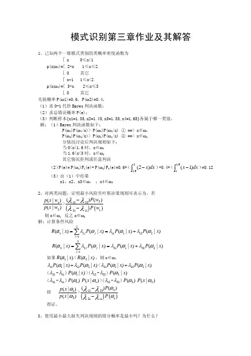
答:不是最小的。首先要明确当我们谈到最小最大损失判决规则时,先验概率是未知的, 而先验概率的变化会导致错分概率变化, 故错分概率也是一个变量。 使用最小最大损 失判决规则的目的就是保证在先验概率任意变化导致错分概率变化时, 错分概率的最 坏(即最大)情况在所有判决规则中是最好的(即最小)。 4、 若 λ11 = λ22 =0, λ12 = λ21 ,证明此时最小最大决策面是来自两类的错误率相等。 证明:最小最大决策面满足 ( λ11 - λ22 )+( λ21 - λ11 ) 容易得到
λ11 P(ω1 | x) + λ12 P(ω2 | x) < λ21 P(ω1 | x) + λ22 P(ω2 | x) ( λ21 - λ11 ) P (ω1 | x) >( λ12 - λ22 ) P (ω2 | x) ( λ21 - λ11 ) P (ω1 ) P ( x | ω1 ) >( λ12 - λ22 ) P (ω2 ) P ( x | ω2 ) p( x | ω1 ) (λ 12 − λ 22) P(ω2 ) > 即 p( x | ω2 ) ( λ 21 − λ 11) P (ω1 )
6、设总体分布密度为 N( μ ,1),-∞< μ <+∞,并设 X={ x1 , x2 ,… xN },分别用最大似然 估计和贝叶斯估计计算 μ 。已知 μ 的先验分布 p( μ )~N(0,1)。 解:似然函数为:
∧Байду номын сангаас
L( μ )=lnp(X|u)=
∑ ln p( xi | u) = −
i =1
N
模式识别第三章作业及其解答
模式识别大作业02125128(修改版)
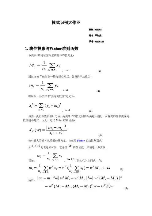
模式识别大作业班级 021252 姓名 谭红光 学号 021251281.线性投影与Fisher 准则函数各类在d 维特征空间里的样本均值向量:∑∈=ik X x kii xn M 1,2,1=i (1)通过变换w 映射到一维特征空间后,各类的平均值为:∑∈=ik Y y kii yn m 1,2,1=i (2)映射后,各类样本“类内离散度”定义为:22()k ii k i y Y S y m ∈=-∑,2,1=i (3)显然,我们希望在映射之后,两类的平均值之间的距离越大越好,而各类的样本类内离散度越小越好。
因此,定义Fisher 准则函数:2122212||()F m m J w s s -=+ (4)使FJ 最大的解*w 就是最佳解向量,也就是Fisher 的线性判别式. 从)(w J F 的表达式可知,它并非w 的显函数,必须进一步变换。
已知:∑∈=ik Y y kii yn m 1,2,1=i , 依次代入上两式,有:i TX x ki Tk X x Ti i M w x n w x w n m ik ik ===∑∑∈∈)1(1,2,1=i (5) 所以:221221221||)(||||||||M M w M w M w m m T T T -=-=-w S w w M M M M w b T T T =--=))((2121 (6)其中:Tb M M M M S ))((2121--= (7)bS 是原d 维特征空间里的样本类内离散度矩阵,表示两类均值向量之间的离散度大小,因此,b S 越大越容易区分。
将(4.5-6)i Ti M w m =和(4.5-2)∑∈=ik X x kii xn M 1代入(4.5-4)2iS 式中:∑∈-=ik X x iT k T i M w x w S 22)(∑∈⋅--⋅=ik X x Tik i k T w M x M x w ))(( w S w i T= (8)其中:T iX x k i k i M x M x S ik ))((--=∑=,2,1=i (9)因此:w S w w S S w S S w T T =+=+)(212221 (10)显然:21S S S w += (11)w S 称为原d 维特征空间里,样本“类内离散度”矩阵。
模式识别作业二

第二次模式识别作业无意中画出来的:x=0:0.01:pi; y=0.5*sin(x);h=plot(x,y,'k');hold onpatch(get(h,'ydata'),get(h,'xdata'),'r')patch(get(h,'xdata'),get(h,'ydata'),'r')patch(-get(h,'xdata'),get(h,'ydata'),'r')patch(-get(h,'xdata'),-get(h,'ydata'),'r')patch(get(h,'xdata'),-get(h,'ydata'),'r')patch(get(h,'ydata'),-get(h,'xdata'),'r')patch(-get(h,'ydata'),-get(h,'xdata'),'r')patch(-get(h,'ydata'),get(h,'xdata'),'r')hold off;3. 用感知器算法求下列模式分类的解向量w:ω1:0,0,0,1,0,0,1,0,1,1,1,0ω2:0,0,1,0,1,1,0,1,0,1,1,1设W(1)=(-1,-2,-2,0),绘出其判别面。
(3,-2,-3,1)代码:%直接增广、正则化xx=[0,0,0,1;1,0,0,1;1,0,1,1;1,1,0,1;0,0,1,1;0,1,1,1;0,1,0,1;1,1,1,1];%原增广矩阵xx(5:8,:)= - xx(5:8,:);%正则化x=xx';w=[-1,-2,-2,0];%初始wflag=0;while flag==0s=w*x%显示分类结果l=find(s<=0);n=length(l) ;if n==0%没有错分向量,结束迭代flag=1;elsefor i=1:nw=w+x(:,l(i))';endendw%显示修正后的wend%draw the picturey=xx(1:24);%去增广y=reshape(y,8,3);y(5:8,:)= - y(5:8,:);%反正则化plot3(y(:,1),y(:,2),y(:,3),'r*');hold onplot3(y(:,1),y(:,2),y(:,3),'ro');grid on[x1,x2]=meshgrid(-1:0.01:1);x3=-(w(1)*x1+w(2)*x2+w(4))/w(3); mesh(x1,x2,x3);hold off;xlabel('x1','fontsize',20);ylabel('x2','fontsize',20);zlabel('x3','fontsize',20);结果:总共进行了6次迭代,最终w=(4 -4 -4 3)。
模式识别作业Homework#2
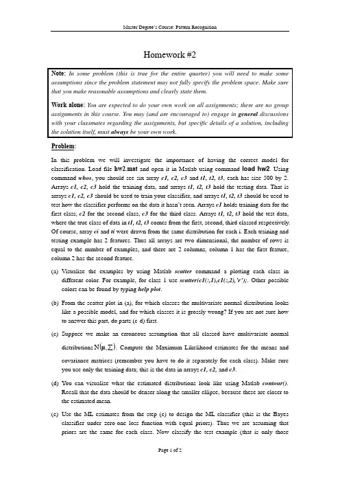
Homework #2Note:In some problem (this is true for the entire quarter) you will need to make some assumptions since the problem statement may not fully specify the problem space. Make sure that you make reasonable assumptions and clearly state them.Work alone: You are expected to do your own work on all assignments; there are no group assignments in this course. You may (and are encouraged to) engage in general discussions with your classmates regarding the assignments, but specific details of a solution, including the solution itself, must always be your own work.Problem:In this problem we will investigate the importance of having the correct model for classification. Load file hw2.mat and open it in Matlab using command load hw2. Using command whos, you should see six array c1, c2, c3 and t1, t2, t3, each has size 500 by 2. Arrays c1, c2, c3 hold the training data, and arrays t1, t2, t3 hold the testing data. That is arrays c1, c2, c3 should be used to train your classifier, and arrays t1, t2, t3 should be used to test how the classifier performs on the data it hasn’t seen. Arrays c1 holds training data for the first class, c2 for the second class, c3 for the third class. Arrays t1, t2, t3 hold the test data, where the true class of data in t1, t2, t3 comes from the first, second, third classed respectively. Of course, array ci and ti were drawn from the same distribution for each i. Each training and testing example has 2 features. Thus all arrays are two dimensional, the number of rows is equal to the number of examples, and there are 2 columns, column 1 has the first feature, column 2 has the second feature.(a)Visualize the examples by using Matlab scatter command a plotting each class indifferent color. For example, for class 1 use scatter(c1(:,1),c1(:,2),’r’);. Other possible colors can be found by typing help plot.(b)From the scatter plot in (a), for which classes the multivariate normal distribution lookslike a possible model, and for which classes it is grossly wrong? If you are not sure how to answer this part, do parts (c-d) first.(c)Suppose we make an erroneous assumption that all classed have multivariate normalNμ. Compute the Maximum Likelihood estimates for the means and distributions()∑,covariance matrices (remember you have to do it separately for each class). Make sure you use only the training data; this is the data in arrays c1, c2, and c3.(d)You can visualize what the estimated distributions look like using Matlab contour().Recall that the data should be denser along the smaller ellipse, because these are closer to the estimated mean.(e)Use the ML estimates from the step (c) to design the ML classifier (this is the Bayesclassifier under zero-one loss function with equal priors). Thus we are assuming that priors are the same for each class. Now classify the test example (that is only thoseexamples which are in arrays t1, t2, t3). Compute confusion array which has size 3 by 3, and in ith row and jth column contains the number of examples fro which the true class isi while the class your classifier gives is j. Note that all the off-diagonal elements in theconfusion array are errors. Compute the total classification error, easiest way to do it is to use Matlab function sum() and trace().(f)Inspect the off diagonal elements to see if which types of error are more common thanothers. That should give you an idea of where the decision boundaries lie. Now plot the decision regions experimentally (select a fine 2D grid, classify each point on this grid, and plot the class with distinct color). If you love solving quadratic systems of equations, you can find the decision boundaries analytically. Using your decision boundaries, explain why some errors are more common than others.(g)If the model assumed for the data is wrong, than the ML estimate of the parameters arenot even the best parameters to use for classification with that wrong model. That is because the multivariate normal is the wrong distribution to use with out data, the MLE parameters we computed in part (c) are not the ones which will give us the best classification with our wrong model. To confirm this, find parameters for the means and variances (you can change as many as you like, from one to all) which will give better classification rate than the one you have gotten in part (e). Hint: it pays to try to change covariance matrices, rather than the means.(h)Now let’s try to find a better model for our data. Notice that to determine the class of apoint; it is sufficient to consider the distance of that point from the origin. The distance from the origin is very important for classifying our data, while the direction is totally irrelevant. Convert all the training and testing arrays to polar coordinates using Matlib function cart2pol(). Ignore the first coordinate, which is the angle, and only use the second coordinate, which is the radius (or distance from the origin). Assume now that all classes come from normal distribution with unknown mean and variance. Estimate these unknown parameters using ML estimation again using only the training data (the arrays ci’s). Test how this new classifier works using the testing data (the arrays ti’s) by computing the confusion matrix and the total classification error. How does this classifier compare with the one using the multivariate normal assumption and why is there a difference?(i)Experimentally try to find better parameters than those found by ML method for classifierin (h). If you do find better parameters, do they lead to a significantly better classification error? How does it compare to part (g)? Why can’t you find significantly better parameters than MLE for the classifier in (h)?。
模式识别作业
模式识别作业图像处理与模式识别作业二题目一:计算特征矢量之间的距离:任意构造10个人在程序设计、离散数学、数据结构、计算机组成原理4门课的成绩表。
计算两两之间的欧式距离、绝对值距离,设计合适的阈值,能否进行分类?答:题目中每个人共有四门课,也就是每个人有4个特征,每门课的成绩也就是这4个特征的量化。
例如某人的成绩就可以表示为(95,68,78,85)这样的一个四维向量。
在这样一个四维空间里,每个个体的相似程度也就可以用欧式距离或者绝对值距离表示。
根据这个相似度,我们就可以将相似度近的分为几类,使其类间距离和最大,类内距离和最小。
或者规定产生几类,具体进行分类。
可用的分类方法有很多,例如最大最小距离法、谱系聚类法、C-均值。
题目二:关于类的定义:如何定义类内各个样本的平均距离?如何定义类之间的距离?答:(1)根据不同的要求类内各个样本的平均距离可以有不同的定义方式。
一般而言,采用先求取类的类心,通过求各个样本与类心距离的平均值.但有时对于样本的聚簇要求格外看中,可以求样本两两距离的和的平均值。
(2)类间距离的方法有很多,例如欧式距离、马氏距离、明氏距离、汉明距离、角度相似性函数。
其中欧式距离较为常用。
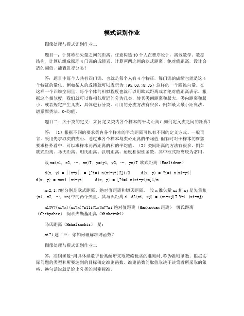
设x=(x1, x2, …, xn)T, y=(y1, y2, …, yn)T 欧式距离(Euclidean)d(x, y) = ||x-y|| = [?i=1 n(xi-yi)2]1/2 d(x, y) = ?i=1 n|xi-yi|d(x, y) = maxi |xi-yi| d(x, y) = [?i=1 n(xi-yi)m]1/mm=2,1,?时分别是欧式距离、绝对值距离和切氏距离。
设n维矢量xi和xj是矢量集{x1, x2, …, xn}中的两个矢量,其马氏距离d d2(xi, xj) = (xi-xj)T V-1 (xi-xj)n1TV?(xi?x)(xi?x)?n11i?1x?m??xi绝对值距离(Manhattan距离)切氏距离(Chebyahev)闵科夫斯基距离(Minkowski)马氏距离(Mahalanohis)是:mi?1题目三:你如何理解准则函数?图像处理与模式识别作业二答:准则函数-用具体函数评价系统所采取策略优劣的准则时,称为准则函数。
模式识别习题及答案
模式识别习题及答案模式识别习题及答案【篇一:模式识别题目及答案】p> t,方差?1?(2,0)-1/2??11/2??1t,第二类均值为,方差,先验概率??(2,2)?122???1??1/21??-1/2p(?1)?p(?2),试求基于最小错误率的贝叶斯决策分界面。
解根据后验概率公式p(?ix)?p(x?i)p(?i)p(x),(2’)及正态密度函数p(x?i)?t(x??)?i(x??i)/2] ,i?1,2。
(2’) i?1基于最小错误率的分界面为p(x?1)p(?1)?p(x?2)p(?2),(2’) 两边去对数,并代入密度函数,得(x??1)t?1(x??1)/2?ln?1??(x??2)t?2(x??2)/2?ln?2(1) (2’)1?14/3-2/3??4/32/3??1由已知条件可得?1??2,?1,?2??2/34/3?,(2’)-2/34/31设x?(x1,x2)t,把已知条件代入式(1),经整理得x1x2?4x2?x1?4?0,(5’)二、(15分)设两类样本的类内离散矩阵分别为s1??11/2?, ?1/21?-1/2??1tt,各类样本均值分别为?1?,?2?,试用fisher准(1,0)(3,2)s2-1/21??(2,2)的类别。
则求其决策面方程,并判断样本x?解:s?s1?s2??t20?(2’) ??02?1/20??-2??-1?*?1w?s()?投影方向为12?01/22?1? (6’) ???阈值为y0?w(?1??2)/2??-1-13 (4’)*t2?1?给定样本的投影为y?w*tx??2-1?24?y0,属于第二类(3’) ??1?三、(15分)给定如下的训练样例实例 x0 x1 x2 t(真实输出) 1 1 1 1 1 2 1 2 0 1 3 1 0 1 -1 4 1 1 2 -1用感知器训练法则求感知器的权值,设初始化权值为w0?w1?w2?0;1 第1次迭代2 第2次迭代(4’)(2’)3 第3和4次迭代四、(15分)i. 推导正态分布下的最大似然估计;ii. 根据上步的结论,假设给出如下正态分布下的样本,估计该部分的均值和方差两个参数。
a2 模式识别第二次作业-推荐下载
模式识别作业报告组员:2011302265 孔素瑶2011302268 马征2011302273 周昳慧1、实验目的(1)试验非参数估计,体会与参数估计在适用情况、估计结果方面的异同。
(2)试验直接设计线性分类器的方法,与基于概率密度估计的贝叶斯分类器进行比较。
(3)体会留一法估计错误率的方法和结果。
2、具体做法(1)挑选上次实验中的一种情况(特征、先验概率等),改用Parzen 窗法或者kn 近邻法估计概率密度函数,得出贝叶斯分类器,对测试样本进行测试,比较与参数估计基础上得到的分类器和分类性能的差别。
(2)同时采用身高和体重数据作为特征,用Fisher 线性判别方法求分类器,将该分类器应用到训练和测试样本,考察训练和测试错误情况。
将训练样本和求得的决策边界画到图上,同时把以往用Bayes 方法求得的分类器也画到图上,比较结果的异同。
(3)选择上述Bayes 分类器和Fisher 分类器,用留一法在训练集上估计错误率,与在测试集上得到的错误率进行比较。
3、实验原理1、挑选身高为特征,选择先验概率为男生0.75女生0.25的一组用Parzen 窗法来求概率密度函数,再用贝叶斯分类器进行分类。
本次实验我们组选用的是正态函数窗:21()2u u φ⎧⎫=-⎨⎬⎩⎭窗宽为h 是调节的参量,N 是样本个数) ,(d 表示维度)。
/N h h =dN N V h =因为区域是一维的,所以体积为。
N n V h =Parzen 公式为:。
()ˆNP x =111Nii N Nx x NV h φ=⎛⎫- ⎪⎝⎭∑女生的条件概率密度为:11111111N i i n x x p N VN h φ=⎛⎫-= ⎪⎝⎭∑ 男生的条件概率密度为:21112222N i i n x x p N VN h φ=⎛⎫-= ⎪⎝⎭∑根据贝叶斯决策规则:(基于类条件概率密度函数)()()()()()1122g x p x w p w p x w p w =-若>0,则判断其为女生,反之为男生。
中科院模式识别第二次作业参考答案
4
当 2 3 时,有:
Q( , 0 ) 不存在。
对分布进行归一化,有 P ( x2 ) ~ U (0, 2 ) ,故
P( x )dx
2
2
1
对 P ( x1 ) ,有
p( x1 )dx1
0 0
1
1
e 1x1 dx1 1
因此, 1 1 。
2
1 ( x )2 1 1 x v 2 exp 2 2 nh 2 hn 2 2 hn 2 n 2 hn hn hn nhn hn nhn 1 ( x )2 exp 2 2 2 2 hn 2 2 hn 1 1 ( x )2 1 exp 2 2 2
(c) 用递归公式计算样本均值,每次更新的计算复杂度为: O ( d ) 用递归公式计算样本协方差,每次更新的计算复杂度为: O ( d ) (d) 当样本量非常大,或者样本是边输入边分类的时候,考虑采用递归公式,这是在线分类。 当样本量比较小,可以全部输入之后再分类的时候,考虑采用非递归公式,这是离线分类。
2
2
)1 。
当 1 1, 2 3 时,取得最大值: Q ( , 0 ) 8.52 故,当 3 时, Q( , 0 ) 取得最大值。
1
1 2 x1 2 e (c) 当 4 时,有 P ( x1 , x2 ) 8 0
因此: pn ( x) ~ N ( , hn )
(b) 计算得:
Var [ pn ( x)] Var [
1 nhn
模式识别大作业(二)
模式识别大作业(二)————C-均值算法与模糊C 均值聚类的比较姓名:谭红光 学号:02125128 班级:021252一 原理:1.C 均值的原理:C 均值聚类算法是一种典型的无监督动态聚类算法。
该算法是在类别数目已知(=k )的条件下进行的,能够使聚类结果的距离平方和最小,即算法的基础是误差平方和准则。
其基本过程是建立初始的聚心和聚类,通过多次迭代,逐渐调整各类的聚心和各像元的类别,直至得到聚类准则约束下的最好结果为止。
本实验的具体过程如下:选择初始类别中心,假设有c 个类别,设置其中心分别为(1)(1)(1)12,,,c Z Z Z 在第k 步迭代中,对于任何一个像元x(是一个N 维向量,N 是高光谱图像的波段数目),按如下方法把它调整到。
各类别中的某一个类别中去。
令d(x ,y)为向量x ,y 之间的距离,若:()()(,)(,)k k i jd x Z d x Z <=, j = 1 2 … c (j i ≠) 则()k i x S∈,其中()k i S 是以()k iZ 为中心的类。
由上一步得到的()k iS(i =1 2…c )个类别新的中心(1)k i Z +()(1)1k i k ix S iZxN +∈=∑其中N i是类别()k iS 的数目。
(1)k i Z +是按照最小J 的原则,J 的表达式为:()(1)1(,)k i ck i i x S J d x Z +=∈=∑∑对所有的i =1 2…c 。
如果,(1)()k k i i Z Z +=,则迭代结束(在程序中,则按照每个类别的对应的那些像素不再变化,则停止迭代),否则转到第二步继续迭代。
2.模糊C 均值的原理在数字图像由于存在混合像素的原因,也就是说一个像素中不仅存在一类地物,因而采用硬分类方式往往不合适,而模糊C 均值就是引入模糊集对每个像素的划分概率不单单是用0或1这样的硬分类方式,而是0和1之间的范围内(包括0和1)。
模式识别习题及答案
模式识别习题及答案模式识别习题及答案模式识别是人类智能的重要组成部分,也是机器学习和人工智能领域的核心内容。
通过模式识别,我们可以从大量的数据中发现规律和趋势,进而做出预测和判断。
本文将介绍一些模式识别的习题,并给出相应的答案,帮助读者更好地理解和应用模式识别。
习题一:给定一组数字序列,如何判断其中的模式?答案:判断数字序列中的模式可以通过观察数字之间的关系和规律来实现。
首先,我们可以计算相邻数字之间的差值或比值,看是否存在一定的规律。
其次,我们可以将数字序列进行分组,观察每组数字之间的关系,看是否存在某种模式。
最后,我们还可以利用统计学方法,如频率分析、自相关分析等,来发现数字序列中的模式。
习题二:如何利用模式识别进行图像分类?答案:图像分类是模式识别的一个重要应用领域。
在图像分类中,我们需要将输入的图像分为不同的类别。
为了实现图像分类,我们可以采用以下步骤:首先,将图像转换为数字表示,如灰度图像或彩色图像的像素矩阵。
然后,利用特征提取算法,提取图像中的关键特征。
接下来,选择合适的分类算法,如支持向量机、神经网络等,训练模型并进行分类。
最后,评估分类结果的准确性和性能。
习题三:如何利用模式识别进行语音识别?答案:语音识别是模式识别在语音信号处理中的应用。
为了实现语音识别,我们可以采用以下步骤:首先,将语音信号进行预处理,包括去除噪声、降低维度等。
然后,利用特征提取算法,提取语音信号中的关键特征,如梅尔频率倒谱系数(MFCC)。
接下来,选择合适的分类算法,如隐马尔可夫模型(HMM)、深度神经网络(DNN)等,训练模型并进行语音识别。
最后,评估识别结果的准确性和性能。
习题四:如何利用模式识别进行时间序列预测?答案:时间序列预测是模式识别在时间序列分析中的应用。
为了实现时间序列预测,我们可以采用以下步骤:首先,对时间序列进行平稳性检验,确保序列的均值和方差不随时间变化。
然后,利用滑动窗口或滚动平均等方法,将时间序列划分为训练集和测试集。